Without special precautions, binary search trees can become arbitrarily unbalanced, leading to O(N) worst-case times for operations on a tree with N nodes. If we keep a binary tree perfectly balanced, lookup with have O(log N) complexity, but insertion or deletion may require completely rearranging the tree to maintain balance, leading to O(N) worst time. A 2-3 tree is required to be completely balanced (all paths from the root to leaves have exactly the same length), but some slack is built in by allowing internal nodes to have 2 or 3 children. This slack allows the balance condition to be maintained while only requiring adjustments on or near the path from the root to the leaf being added or removed. Since this path has length O(log N) and each adjustment take time O(1), the total time for insertion or deletion, including adjustments, is O(log N).
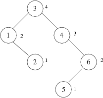
A different approach is taken by AVL trees (named after their inventors, Russians G.M. Adelson-Velsky and E.M. Landis). An AVL tree is a binary search tree that is "almost" balanced. Recall that the height of a tree is the number of nodes on the longest path from the root to a leaf. We will say that an empty tree has height 0. With this convention, the height of a non-empty tree is one greater than the maximum height of its two subtrees. A binary search tree is an AVL tree if there is no node that has subtrees differing in height by more than 1. For example,
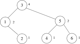
is a binary search tree, but it is not an AVL tree because the children of node 4 have heights 0 (empty) and 2. The height of each node is written next to it so you can see that node 4 is the only node that violates the AVL condition in this case. By rearranging node 4 and its descendents, we convert this tree into a binary search tree with the same data, which satisfies the AVL condition.
A perfectly balanced binary tree is an AVL tree. If it has N nodes, its height is log2(N + 1). What is the worst possible (most unbalanced) AVL tree of height h? It is Th defined as follows: T0 is the empty tree, and T1 is the tree containing a single node. For h > 1, Th has one node at the root with two children, the trees Th-1 and Th-2. Here is a picture of T4:
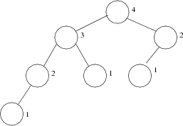
We have omitted the keys but indicated the heights of the subtrees. Note that each non-leaf node has a left subtree that is one level higher than its right subtree. How many nodes are there in Th? First let's count leaves. If fn is the number of leaves in Tn, then f0 = 0, f1 = 1, and for h > 1, fh = fh-1 + fh-2. Thus the fh numbers are the famous Fibonacci numbers. In fact the trees Th defined above are sometimes called Fibonacci trees. The number of internal nodes in a binary tree is always one less than the number of the leaves (can you see why?), so the number of nodes in Th is approximately 2 fn. The Fibonacci numbers fh are known to grow as an exponential function of h, so the height of Th grows logarithmically with the number of nodes. In fact, it can be shown that the height of an AVL tree with N nodes is bounded by 1.44 log2 N. In other words, the worst possible AVL tree is less then 1-1/2 times has high as the best possible. In particular, the time for lookup in an AVL tree of size N is O(log N).
Adding or removing a leaf from an AVL tree may make many nodes violate the AVL balance condition, but each violation of AVL balance can be restored by one or two simple changes called rotations.
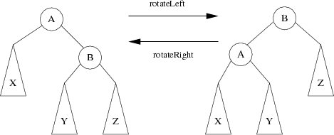
If the tree on the left is a binary search tree, the keys in subtree X are less than A, the keys in tree Z are greater than B, and the keys in Y are between A and B. Thus the tree on the right also obeys the ordering restriction on binary search trees. The code for rotateLeft actually quite simple:
/** Rotates node a to the left, making its right child into its parent.
 * @param a the former parent
 * @return the new parent (formerly a's right child)
 */
Node rotateLeft(Node a) {
    Node b = a.getRight();
    a.setRight(b.getLeft());
    b.setLeft(a);
    return b;
}
The code for rotateRight is similar (can you write it?).
Consider what happens when you add a new leaf to an AVL tree. If you're lucky, the tree will still have the AVL balance property. If not, a little thought should convince you that any violations of the property must be on the path from the root to the new leaf. Let n be the lowest node that violates the AVL property and let h be the height of its shorter subtree. The tree was an AVL tree before the new leaf was added, and adding a leaf to a tree adds at most one to its height, so the height of the taller subtree must now be h + 2, and the new leaf was added as a descendent of one of n's grandchildren. There thus four cases we need to consider. In the first case, the new leaf was added under n.left.left.
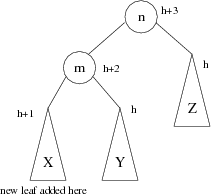
In this case, a single right rotation leads to this:
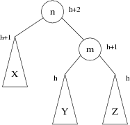
Note that the AVL violation at node n has gone away. In fact, node n and m are now completely balanced. The second case, in which the new leaf was added under n.left.right is a bit more complicated.
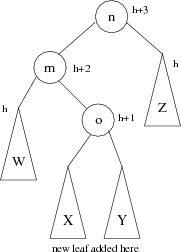
Here one of trees X and Y has height h and the other has height h - 1. Here's what happens if we do a left rotation at node m followed by a right rotation at node n:
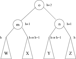
Once again, all AVL violations under node n have been repaired. The remaining two cases (the new leaf was added under n.right.left or under n.right.right) are completely symmetrical, and are left as an exercise for the interested reader (you!).
What's the worst-case complexity for insertion? The code walks down the tree from the root to find where the new leaf goes and adds it (time O(log N)). Then, on the way back up (in the program, this code will be after the recursive call returns), it looks for AVL violations and fixes them with rotations. Since a constant (O(1)) amount of work is done at each node along the path, the total amount of work is proportional to the length of the path, which is O(log N). There's one more coding detail to consider. This analysis assumes we can determine the height of a node in time O(1). To do this, we need to add a height field to each node and update it whenever it changes. The only time the height of a node changes is when a leaf is added below it or when it is involved in a rotation. Thus all height changes are on the path from the root to the new leaf, each change has code O(1), and all the height maintenance adds at most O(log N) to the cost of insertion.
Binary search trees guarantee O(h) worst-case complexity for lookup, insertion, and deletion, where h is the height of the tree. Unless care is taken, however, the height h may be as bad as N, the number of nodes. We have considered two ways of ensuring that trees stay well enough balanced so that the height, and hence the running time of operations, is O(log N). 2-3 trees require that all paths from the root to leaves are exactly the same length, but allow internal nodes to have two or three children. AVL trees require the heights of the subtrees of any node to differ by no more than one level, which ensures that the height is O(log N). Red-black trees can be viewed as an implementation of 2-3 trees that represents each 3-node as a pair of binary nodes, one red and one black. It can also be viewed as variation on AVL trees. Whereas AVL trees are binary trees with a height field in each node and insert and delete operations restructure the tree to ensure restrictions on heights, red-black trees are binary trees with a red bit in each node and operations that restructure (and re-color) nodes to ensure restrictions on colors. The height of an AVL tree is bounded by roughly 1.44 * log2 N, while the height of a red-black tree may be up to 2 * log2 N. Thus lookup is slightly slower on the average in red-black trees. On the other hand, it can be shown that whereas an insertion in an AVL tree may require O(log N) rotations, an insertion in a red-black tree requires only O(1) corresponding operations. O(log N) work is necessary anyhow to decide where to add the new leaf, so both kinds of tree have the same overall complexity, but the constant bound on restructuring operations in red-black trees affects certain advanced applications that are beyond the scope of this discussion.