Phylogenetic Trees

We now begin Unit Two, in which we will be discussing phylogenetic trees.

“Phylogenetic” has two roots:

• Phylo: "type, kind, race, or tribe"
• Genetikos: "referring to origin" (genes)

“the origin of types”

Phylogenetic trees are the “evolutionary trees” that you see in science museums and nature shows.

• Shows how many species are related.
• Diverge from a common ancestor.
• Commonly presumed that far enough back, all known life had a single origin.

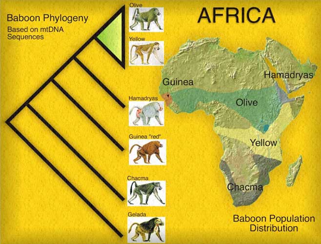
Here's a sample phylogenetic tree for baboons:

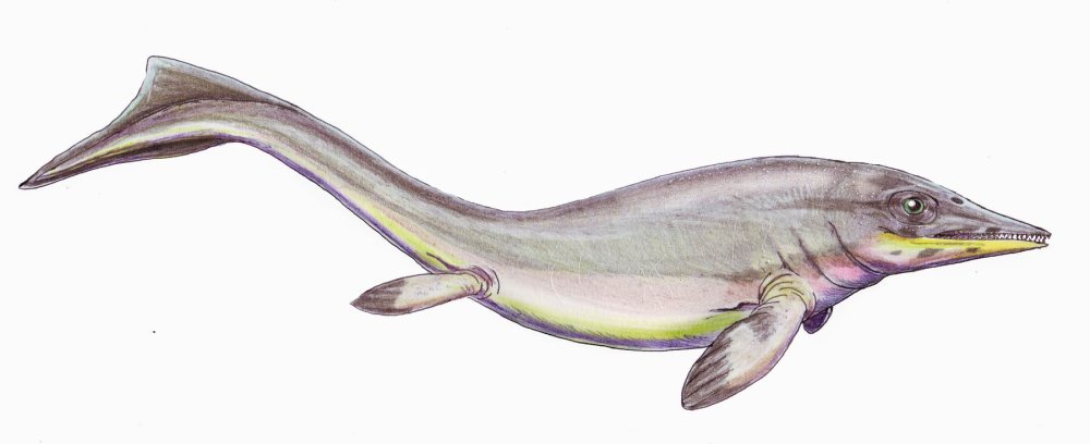
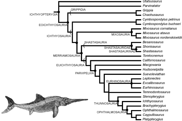
Here's another one for icthyosaurs:

Phylogenetic trees don't need to be based on species.

• You've already seen a tree based on a family of proteins: globins.
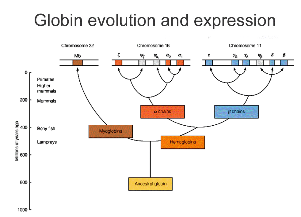
• Can actually use the evolution of proteins and specific sequences of DNA to sketch out how species are related.
• In fact, “species trees” that are generated are often consensus trees from looking at several different features and sequences.
• Can also look at mitochondrial DNA (mtDNA).
  • Matrilineal—no sexual recombination.
  • Higher mutation rate than nuclear DNA.
  • Often used to discriminate species. (Look closely at the baboon tree.)

From these examples, we see that the following holds true:

• The leaves represent things (genes, individuals/strains, species) being compared.
  • The term taxon (taxa plural) is used to refer to these when they represent species and broader classifications of organisms.
• Internal nodes are hypothetical ancestral units.
• In a rooted tree, path from root to a node represents an evolutionary path.
  • The root represents the common ancestor.

Some trees do not have a well-defined common ancestor.

• We calls these unrooted trees.
• An unrooted tree specifies relationships among things, but not evolutionary paths.

Constructing Phylogenetic Trees

The basic task:

• Given: data characterizing a set of species or genes.
• Do: infer a phylogenetic tree that accurately characterizes the evolutionary lineages among them.

Why construct trees?

• To understand lineage of various species.
• To understand how various functions evolved.
• To inform multiple alignments.
• To identify what is most conserved/important in some class of sequences.

There are three different common goals for constructing a tree:

• Distance: find the tree that accounts for estimated evolutionary distances.
• Parsimony: find the tree that requires minimum number of changes to explain the data.
• Maximum likelihood: find the tree that maximizes the likelihood of the data.

Similarly, trees can be constructed from various types of data.

• Distance-based: measures of distance between species/genes.
• Character-based: morphological features (e.g. # legs),
• DNA/protein sequences: look at how similar different sequences are.
• Gene-order: linear order of corresponding genes in given genomes.
  • Some mutations can rearrange the genome.

Rooted & Unrooted Trees

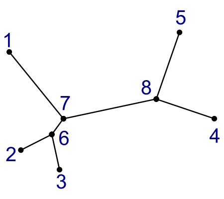
Here are the two kinds of tree:

Unrooted Tree		Rooted Tree

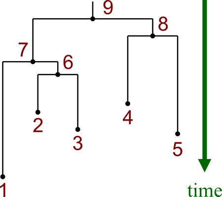Remember:

• Rooted trees tell you something about evolutionary paths over time.
• Unrooted trees only tell you relations.

Notice that these two trees are made from the same data.

• Leaf nodes are numbered 1-5.
• Internal nodes are numbered 6-8.
• Rooted tree has additional node 9, which is the root.

First question: “Given n species/genes/sequences/etc., how many trees is it possible to construct?”

• If it's a reasonable number, a tree-construction algorithm is immediately obvious:
  1. Enumerate every possible tree buildable from the n leaves.
  2. Score each of them, returning the one with the best score.

The solution involves a fair amount of graph theory, and it turns out like this:

Entering numbers into the above formulas, we get the following table:

# Leaves (n)	# Unrooted Trees	# Rooted Trees
4	3	15
5	15	105
6	105	945
8	10,395	135,135
10	2,027,025	34,459,425

In other words:

• This is an exponential function.
• No, it is not a reasonable number.
• We need to have a clever algorithm.

Distance-Based Methods

We start by considering a couple of distance based methods: UPGMA and Neighbor Joining.

We define the problem as follows:

• Given: An n × n matrix M in which M_ij is the distance between objects i and j.
• Do: Build an edge-weighted tree such that the distances between leaves i and j correspond to M_ij.

The basic idea behind a distance based approach is this: the (vertical) distance between any two leaves should correspond to their predefined distance.

UPGMA

One of the most basic examples of such a method is UPGMA.

• Unweighted Pair Group Method using arithmetic Averages.
• Basic idea:
  • Iteratively pick two leaves/clusters and merge them.
  • Create new node in tree for merged cluster.
• Distance d_ij between clusters C_i and C_j is defined as:
  • (Average distance between pairs of elements from each cluster.)

The algorithm runs as follows:

1. Assign each sequence to its own cluster.
2. Define one leaf for each sequence; place it at height 0.
3. While more than two clusters:
   1. Determine two clusters i, j with smallest d_ij.
   2. Define a new cluster C_k by merging C_i and C_j.
   3. Define a node k with children i and j; place it at height (½ d_ij).
   4. replace clusters i and j with k.
   5. Compute distance between k and other clusters.
4. Join last two clusters, i and j, by root at height (½ d_ij).

Fortunately, there's a shortcut to calculating new distances:

• Given a new cluster C_k formed by merging C_i and C_j, the distance to another cluster C_l is:

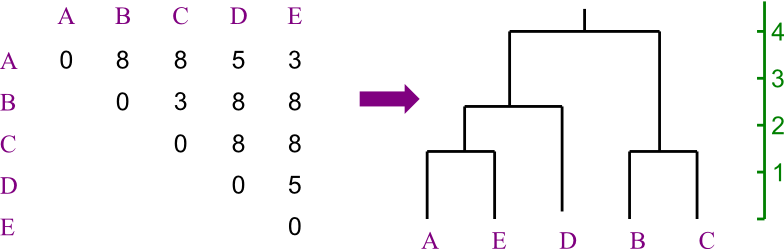
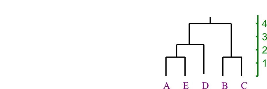
Example

Let us say you are trying to create a phylogenetic tree for five species, labeled A through E. Their distances from each other are given by the following matrix:

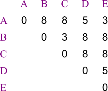
Build the tree using UPGMA.

Solution:
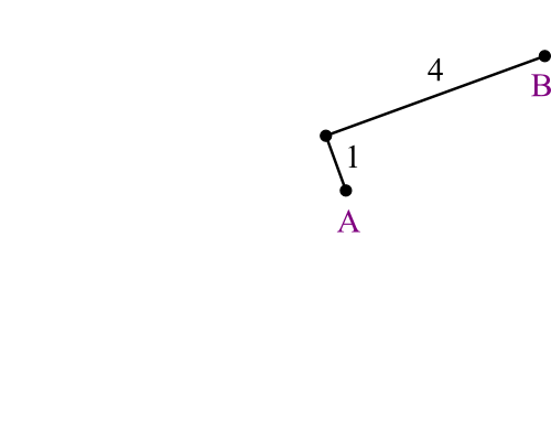
Here's how the problem starts out. 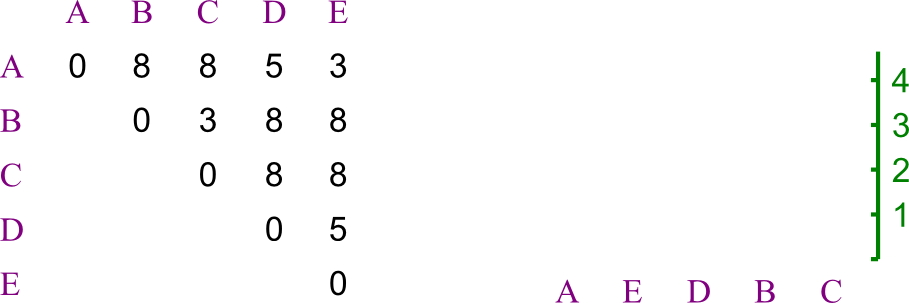First we see which two leaves are closest to each other.

• There's a tie, so we're just going to pick A and E.
• We recalculate the distance matrix, so that AE is a member.
  • Its distances are the averages of those of A and of E.
  • In this case, that's trivial.

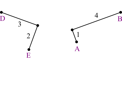
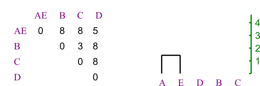Repeating, we chose to merge B and C.

• Again, distances are easy to recompute.

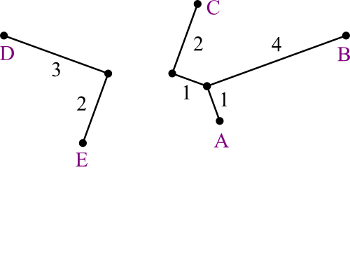
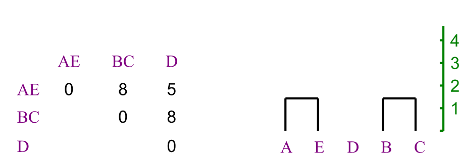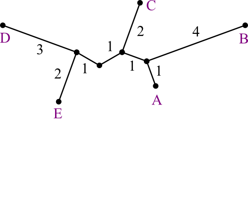
Now AE is closest to D. 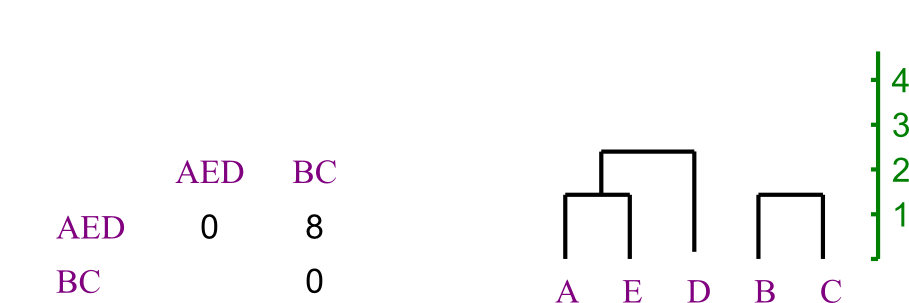And merge the last two, making the tree's root.

You may have noticed that in this example, the distances were remarkably well behaved.

• Averages were easy to calculate—too easy.
• Should be a tip-off that this is toy data.

Actually, this data was constructed using the molecular clock assumption.

• Divergence of elements is assumed to occur at the exact same rate at all points on the tree.
  • “Evolution at a constant rate.”
• This assumption is not generally true. Selection pressures vary across:
  • Time periods
  • Organisms
  • Genes within an organism
  • Regions within a gene
• In other words, things evolve at different rates.
• If this does hold, then the data is said to be ultrametric.
  • Ultrametric data never really occurs in nature.
• Given ultrametric data, UPGMA will reconstruct the tree T that is consistent with the data.

How can you tell ultrametric data?

• For any triplet of elements i, j, and k, one of two things will be true:
  1. The distances are all equal.
  2. Two are equal and the remaining one is smaller.
• For the matrix in the example, this was certainly true:

In general, for real data:

• UPGMA is not guaranteed to return the correct tree.
  • Differing rates of evolution can confound it.
  • Will do better with classic Darwinian evolution than with punctuated equilibrium.
• However, it may still be a reasonable heuristic.

Neighbor Joining

Neighbor Joining is another distance-based method for reconstructing phylogenetic trees from distance data.

• Like UPGMA:
  • Constructs a tree by iteratively joining subtrees.
• Unlike UPGMA:
  • Doesn't make molecular clock assumption.
  • Produces unrooted trees.
  • Assumes additivity: distance between pair of leaves is sum of lengths of edges connecting them.

There are also two key differences in the merging process:

• How pair of subtrees to be merged is selected on each iteration.
• How distances are updated after each merge.

So far, each iteration we've chosen the two clusters that are closest together.

• But suppose the real tree (which is hidden from us) looks like this:

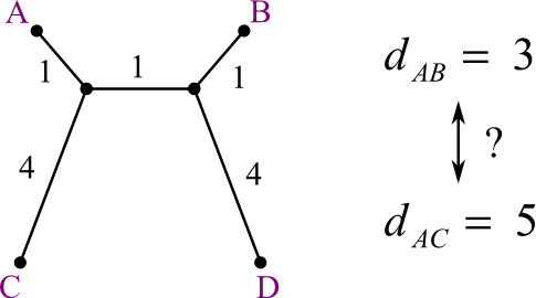
Should A be joined with C or D?

• A and B are closest.
• A and C is the real answer.

How can we make a method that will choose C over B?

• Answer: we penalize merging with clusters that are close to many other clusters.
• Ideally, we join isolated pairs.

Let us define the penalty factor u_i as follows:

• It's almost the average distance to all the other clusters.
  • Divide by 2 less than the total number of clusters.
• A cluster i that is far away from the other clusters will have a high u score.
  • It will be an attractive target for a merge...if another cluster is close enough.

Every iteration, we will merge the two clusters that have the lowest biased distance score D:

When we merge two clusters i and j into a new cluster k, it looks like this:

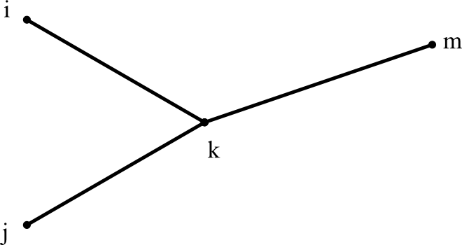
We can find k's distance to any other cluster m using:

This equation corresponds to a situation like this:

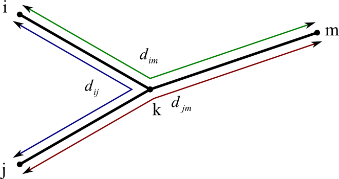
• We already know d_ij, d_im, and d_jm.
  • (We assume all our distances calculated along the paths of the tree.)
• If we add the length of d_im (green path) and d_jm (red path), and then subtract d_ij (blue path), the result is twice the length of d_km.
• So ÷ 2.

The distance from i or j to its new parent is calculated in a similar way:

• Also, d_ik + d_jk = d_ij.

However, it's a little easier to use the u values:

So the total algorithm is as follows:

• So long as there are still more than 2 clusters:
  1. Calculate u value for each cluster.
  2. Calculate the biased distance score for each possible pair.
  3. Pick the pair with the lowest score to merge.
  4. Recalculate all the distances to the new cluster.
     • Note that this changes your u values.
• The last two clusters can just be joined with the given distance.

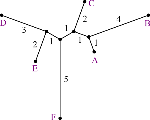
Example

Here is a matrix of distances. Use Neighbor Joining to solve for the tree.

	A	B	C	D	E	F
A	0	5	4	7	6	8
B		0	7	10	9	11
C			0	7	6	8
D				0	5	9
E					0	8
F						0

Solution:

From the matrix, calculate all the u scores. Then calculate the biased distances, and insert the new cluster. Keep going until done.

A B C D E F A 0 5 4 7 6 8 B 0 7 10 9 11 C 0 7 6 8 D 0 5 9 E 0 8 F 0

uA = (5 + 4 + 7 + 6 + 8) ÷ 4 = 7.5 uB = (5 + 7 + 10 + 9 + 11) ÷ 4 = 10.5 uC = (4 + 7 + 7 + 6 + 8) ÷ 4 = 8 uD = (7 + 10 + 7 + 5 + 9) ÷ 4 = 9.5 uE = (6 + 9 + 6 + 5 + 8) ÷ 4 = 8.5 uF = (8 + 11 + 8 + 9 + 8) ÷ 4 = 11

Of all the biased distances, we have a tie:

We'll arbitrarily choose to merge A and B. We need to find each one's distance to its new parent:

We also calculate each other element's distance to AB, and start a new step.

AB C D E F AB 0 3 6 5 7 C 0 7 6 8 D 0 5 9 E 0 8 F 0

uAB = (3 + 6 + 5 + 7) ÷ 3 = 7 uC = (3 + 7 + 6 + 8) ÷ 3 = 8 uD = (6 + 7 + 5 + 9) ÷ 3 = 9 uE = (5 + 6 + 5 + 8) ÷ 3 = 8 uF = (7 + 8 + 9 + 8) ÷ 3 = 10.67

Another tie in the biased distances:

Arbitrarily choose D and E.

Find each one's distance to its new parent:

And do the distances for the next full matrix:

AB C DE F AB 0 3 3 7 C 0 4 8 DE 0 6 F 0

uAB = (3 + 3 + 7) ÷ 2 = 6.5 uC = (3 + 4 + 8) ÷ 2 = 7.5 uDE = (3 + 4 + 6) ÷ 2 = 6.5 uF = (7 + 8 + 6) ÷ 2 = 10.5

The smallest biased distances are:

Join C and AB. Find each one's distance to its new parent:

And do the distances for the next full matrix:

ABC DE F ABC 0 2 6 DE 0 6 F 0

uABC = (2 + 6) ÷ 1 = 8 uDE = (2 + 6) ÷ 1 = 8 uF = (6 + 6) ÷ 1 = 12

We have a 3-way tie in the biased distances:

Arbitrarily choose ABC and DE.

Find each one's distance to its new parent:

And, at long last:

ABCDE F ABCDE 0 5 F 0

The u scores have ÷ 0, but don't matter anyway on the last step.

Just connect ABCDE and F with a distance of 5.

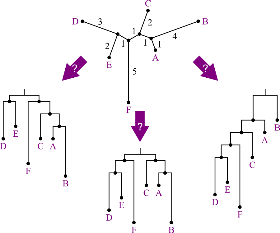
Rooting Unrooted Trees

We just put a lot of effort into joining these taxa into a tree...but it's unrooted.

• Shows relationships, not evolution.
• Rooted tree would be preferable.

But how can we decide who's an ancestor of whom?

• There are several possible answers:

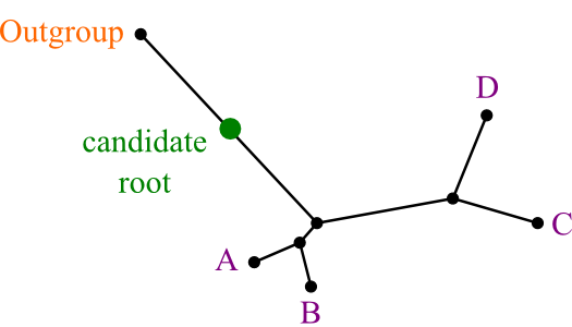
Answer: use an outgroup.

• “A species known to be more distantly related to remaining species than they are to each other.”
• The point where the outgroup joins the rest of the tree is best candidate for root position.

Additivity

So, intuitively, what does additivity mean?

• Not all data makes good trees.
  • If A and B are “siblings” on a tree, most of the paths from them to other taxa are the same.
  • Therefore, good data will always have them differing by the same amount from each other, with respect to all their distances.

  A B C D E F A 0 5 4 7 6 8 B 0 7 10 9 11 C 0 7 6 8 D 0 5 9 E 0 8 F 0

• Additivity means that the data can be used to make a well-behaved tree.

In principle, one might expect high-fidelity data to be additive.

• Of course, data always has noise.
• Evolution sometimes backtracks.
• Horizontal gene transfer can also make non-additive data.

Just like with ultrametric data, there's a test for additive data:

• Consider every set of four leaves, i, j, k, and l.
• There are three ways to pair them off: ij/kl, ik/jl, il/jk.
• Sum the distances between partners: d_ij + d_kl, d_ik + d_jl, d_il + d_jk.
• For these three sums, the data is additive if and only if two are equal, and the third is smaller.

Here's a graphical representation of why this is so:

Neighbor Joining returns the proper tree if the data is additive.

• If not, it's only a heuristic.
• Even so, Neighbor Joining works very well in practice, and is used in many papers.
• Often in conjunction with other methods.

Complexity Analysis

The time and space required to run distance-based tree-building methods relies mainly on the number of taxa in the dataset.

For time complexity:

• We perform (n-1) merges, where n is the number of taxa.
• Each merge must compare O(n²) pairs.
• The overall complexity is thus O(n³).

Before, I hinted that O(n³) may be too slow/too big.

• Fortunately, the number of taxa to relate doesn't grow as quickly as the length of sequences.
• There exist methods to speed up the calculation to O(n²) in many cases.
  • Worst case still O(n³).

If we need to calculate the distances, this is an additional O(n²) step.

• If calculating from sequence data of length s, this step is O(n²s).

For space complexity, we need to store two things:

1. The distance matrix/matrices.
   • Size O(n²).
2. The growing tree.
   • Size O(n).

The total space complexity is thus O(n²).

Parsimony

Distance-based tree methods work fairly well, but they have a flaw.

• Entire sequences are boiled down to a few distances.
• A lot of the data is just thrown away.
• Might we get better results if we do something different?

Parsimony-based methods don't use distance matrices.

• Given: character-based data.
• Do: find tree that explains the data with a minimal number of changes.
  • Uses Occam's Razor.
• Focus is on finding the right tree topology, not on estimating branch lengths.

Example

Given the four entities on the bottom of the each tree, which tree better explains their ancestry?

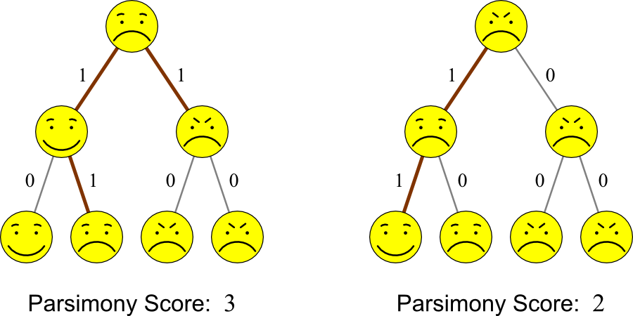
Solution:
Both trees could potentially indicate the ancestry of Smilius familiaris. However, the tree on the right has fewer changes. Therefore, parsimony says that it is the more likely tree.

Here's a slightly less cute example:

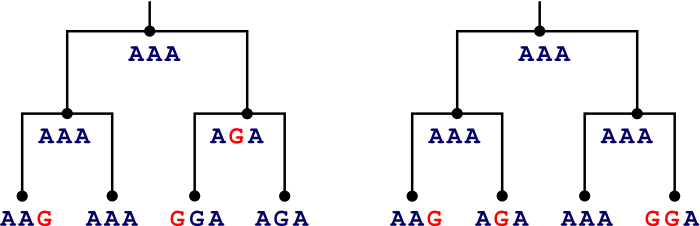
• Parsimony prefers the tree on the left.

One thing that you may have noticed in these examples is that every feature or base/amino acid is independent of all the others.

• This assumption is typical for parsimony approaches.
• Therefore problems are often split into components:
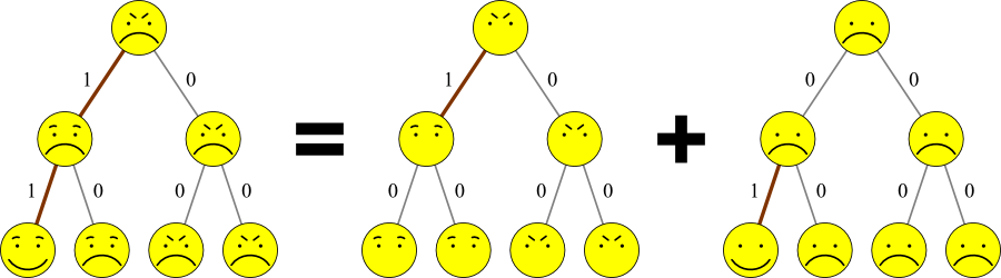
• From now on, examples will only show a single feature or letter.
  • To apply these to larger data sets, do every feature separately and combine them.

Parsimony approaches usually have two different components:

1. Search through many different tree topologies to find a good one.
2. Find the minimum number of changes needed to explain the data, for a given tree topology.

We'll start by focusing on just doing the latter.

• This is sometimes called the small parsimony problem.
• Doing both is likewise called the large parsimony problem.
  • Much more difficult.

Fitch's Algorithm

The simplest parsimony problem to solve is an unweighted small parsimony problem.

• Unweighted: any base can change into another base with equal probability.
• Final score is the sum of base changes.
• Find the tree with the lowest score.

Fitch's Algorithm is the most common solution.

• Published in 1971 by Walter Fitch.
• Assumes that all bases (or other characters) are independent of one another.
  • Solve for each one separately.
• Assumes that the tree is given—we just need to fill in the bases for the ancestor nodes.

Fitch's Algorithm has two main steps:

1. Traverse the tree from leaves to root (“bottom-up”), determining a set of possible states (e.g. nucleotides) for each internal node.
2. Traverse the tree from root to leaves (”top-down”), picking ancestral states from the sets calculated in Step 1.

The first step runs from the leaves up to the root.

• For every node v, let its children be u and w.
• Sets of allowed states of these nodes are likewise called S_v, S_u, and S_w.
• Determine the states in S_v by the following formula:
• The final score is the number of union operations that was needed.
  • This is a count of the minimum number of changes necessary to explain the differences observed.

The second step runs from the root to the leaves.

1. If a node's parent's state is in its own set, pick it.
2. If not (or the node doesn't have a parent), just pick one arbitrarily.

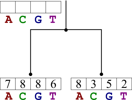
Example

Looking at six related proteins, we conjecture that they are related as in the tree shown below. The base at position 521 is (in the six proteins respectively) C, T, G, T, A, and T. Use Fitch's Algorithm to determine which base was present in the ancestor proteins, back to the root.

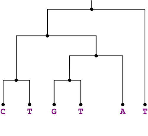
Solution:
Using Fitch's Algorithm, we go through each node bottom-up, determining a set of possible states. Then we go back through top-down, narrowing each down to a single state.

(If this were automated, we'd do the exact same thing for all of the other bases too.)

Complexity Analysis of Fitch's Algorithm

The running time of Fitch's Algorithm depends on 3 things:

1. The number of taxa to be related (n).
2. The number of allowed states for each node (k).
3. The total length of the sequences being compared (s).

The number of taxa determines the number of ancestor nodes.

• Given n taxa, there are (n-1) ancestor nodes.
• Therefore, the time complexity has a linear dependency on the number of taxa.

The number of possible states (e.g. 4 for nucletide bases) is also important in this algorithm.

• We need to check for each one, if it's present in the child nodes.
• “Union” and “intersection” algorithms have a linear dependency on the number of allowed states.
• Therefore, the time complexity is also linearly dependent on k.

Finally, we need to do all of these steps once for each character in the sequences.

• Linear dependency again.

So the total time complexity is O(nks).

• In truth, k is such a minor component that it can be ignored.
• Wouldn't be the case if k were quadratic, or for ridiculously large values of k.

Space complexity is a similar calculation.

• Space complexity is also O(nks).

Sankoff's Algorithm

The weighted small parsimony problem adds a complication:

• Not all state changes are equally likely.
• Use a matrix to represent different costs.

	A	C	G	T
A	0	9	4	3
C		0	4	4
G			0	2
T				0

Sankoff's Algorithm provides an answer.

• Originally credited to David Sankoff (1975).
• Revised by Sankoff with Robert Cedergren (1983).
• Two-step process, like Fitch's Algorithm.
  1. Go up the tree, filling in states.
  2. Go back down, selecting states based on prior calculation.
• In the case of a 0/1 matrix, simplifies to Fitch's Algorithm.

Basic idea:

• Instead of a discrete set at each node, store a table of point values of states.
• The values represent the lowest cost possible for that node, given that it contains that state.
• Calculate a cost for each state for each node from that node's children.

For example, let us assume that a certain node is in state t.

• Its cost is the sum of its children's costs given their states i and j, plus the costs to change i to t and j to t.
• However, we don't really know which states the nodes are in, we have to calculate the costs for all values of i, j, and t.
  • Really, just store the costs for the best i and j for every t.

Formally, the cost table for each leaf is determined by: and the cost table for every other node is given by: where δ_i,t represents the cost to get from state i to state t.

The second step is simple:

• Assign the root to be the state with the lowest cost.
• Assign any internal node to the state that led most efficiently to its parent having its assigned value.
• Very similar to the traceback method used in Needleman-Wunsch.

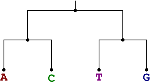
Example

Solve the weighted small parsimony problem for the bases A, C, T, and G related as shown in the tree below. Use the weight matrix shown.

A C G T A 0 9 4 3 C 0 4 4 G 0 2 T 0

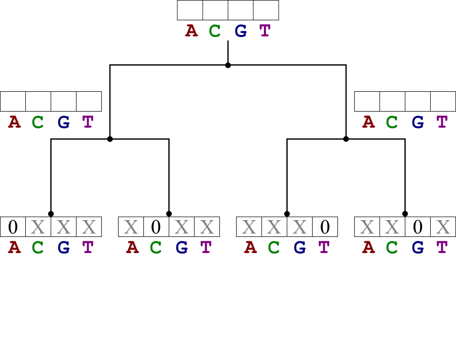
Solution:

Start by filling in the cost tables for the leaf nodes.

• Those entries corresponding to the leaf state have value 0.
• Other entries have value ∞.

Continue upwards to the root, filling in the score tables. Then assign all the nodes the states that lead to the lowest cost at the root.

Complexity Analysis of Sankoff's Algorithm

Complexity analysis is much the same as that for Fitch's Algorithm.

• Time complexity: O(nks).
• Space complexity: O(nks).
• Relation between the two algorithms is evident.

P and NP

Before we get to the large parsimony problem, we need to make another digression into complexity theory.

• Unfortunately, the large parsimony problem is NP-complete.
• What does this mean?

Some problems have polynomial complexity.

• O(n), O(n² log n), even O(n²⁰⁵).
• We call this set of problems P.
• Very roughly, these are “solvable problems”

Other problems are nondeterministically polynomial.

• Basically, they would be polynomial if you could try many solutions at once.

Think of a jigsaw puzzle.

• Difficult problem—it takes a lot of time.
  • Brute force solution: O(n!), where n is the number of pieces.
• But it's really easy to check if you have the right solution.
• So just try all possible solutions at the same time, and pick the one that worked.
• Solving a jigsaw puzzle is thus of nondeterministically-polynomial complexity...it's part of the NP group.

This is part of the reason scientists are so interested in making a quantum computer.

• Computer's memory can store many values simultaneously.
• Could be used to solve an NP problem by trying everything at once.

Many NP problems are logically equivalent to each other.

• It's been proven that if you could solve any one of them in polynomial time, you could solve them all.
• We say that these problems are NP-complete.

As strange as it may seem, no one's actually proven that an NP-complete problem can't be solved in P time.

• Referred to as the P-NP Problem.
• Outstanding problem in computational theory, with a $1,000,000 prize.
• If someone were to solve this, it would have major implications for bioinformatics...as well as cryptography, artificial intelligence, databases, and many other fields of computer science.
• Even though it hasn't been solved, most people think that P≠NP.

But for the purposes of bioinformatics, what it means is this:

• NP and NP-complete problems can't be solved exactly in a reasonable amount of time.
• You need to use a heuristic.

The Large Parsimony Problem

If we're given a tree a priori, finding the most parsimonius ancestors is easy.

• But in real life, we're not given a tree.
• In fact, there's not a known way to “deduce” a tree from the taxa.
• Only way to do it: try many different trees.

As we saw above, trying every tree is unreasonable:

# Leaves (n)	# Unrooted Trees	# Rooted Trees
4	3	15
5	15	105
6	105	945
8	10,395	135,135
10	2,027,025	34,459,425

• This is the “brute force” solution.

We have to search for a good tree.

• Consider one tree at a time.
• After each tree, find a small change to give a better answer.
• Stop when you think you have the best tree.

This is a heuristic approach.

• We're not guaranteed to find the best tree.
• But it cuts time, and we're reasonably sure we have a good one.

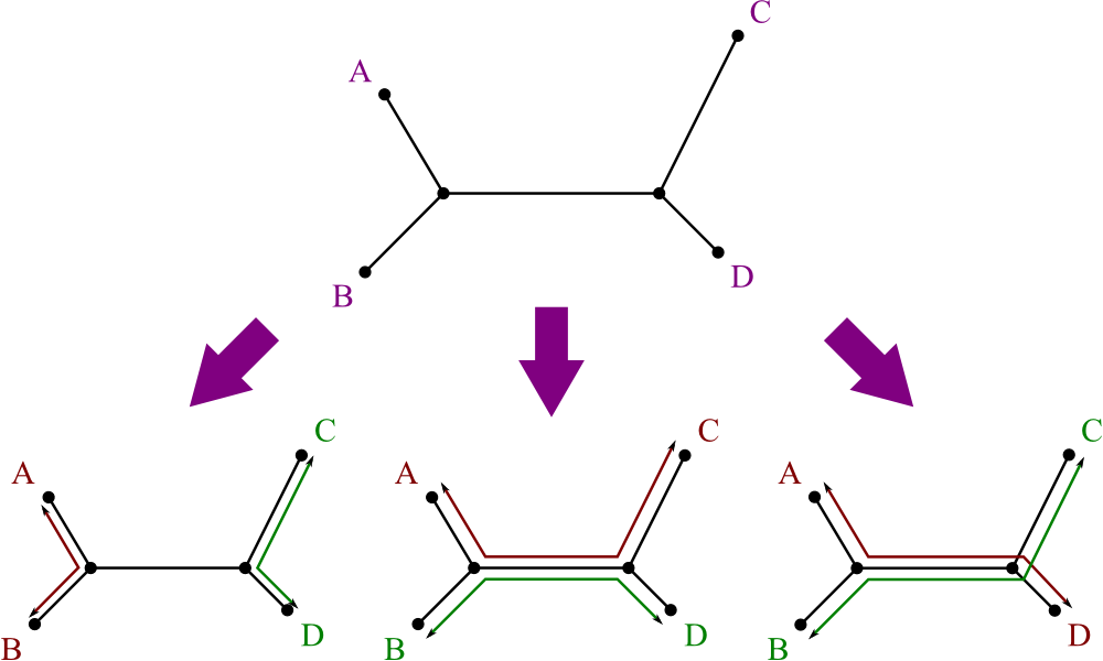
There is a little good news:

• Parsimony usually gives the exact same answer for rooted and unrooted trees.
  • If done right, it always gives the same answer.
• So we only need to search through the unrooted trees, not the rooted ones.

Searching

Say you're in a large old house, and you hear a noise.

• You want to figure out where it's coming from, so you move room-to-room trying to find the source.
• From a room you're in, listen from all the doorways. Walk in the direction you think it's coming from.

Will you find the source?

• Maybe.
• There might be a direct path to the source.
• Or, if you're unlucky, the acoustics will make it seem like the right way to go is the wrong direction.
• Or maybe you went the right direction, but the noise is coming from a different floor. When you get as close as you can, there's no way up.

This is a searching problem.

• Goal: find the noise.
• Search space: the rooms of the house.
• Possible actions: walk to an adjacent room.

The brute force solution would be:

• Go into every room in the house, in turn.
• Report the one that had the loudest noise.
• If the house is too big, this is infeasible.

Searching for Parsimonious Trees

Since we can't look at every tree, we need another approach.

• Searching is a reasonable approach.

Here's how we set up the problem.

• Goal: find the most parsimonius tree.
• Search space: all the possible trees for n taxa.
• Possible actions: slightly change around the current tree.
  • Trees that are only slightly different are considered “neighbors” or “adjacent trees.”.
  • Every time we look at a new tree, we perform the small parsimony problem on it.

Here are the steps to the algorithm:

1. Start with a tree.
2. Do small parsimony on it.
3. Keep doing:
   • Do small parsimony on all neighbors of current tree.
   • Chose neighbor with best cost, and switch to that one.
   • If the current tree had a lower cost than all its neighbors, stop loop.
4. Current tree is best one found.

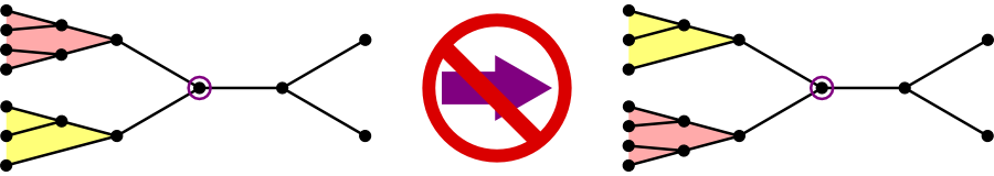
For the current tree, how do we determine which trees are adjacent?

• Note that we can't just switch around the children of a certain node—it would be the same tree!

One idea: pick two nodes from different areas of the tree, and swap them.

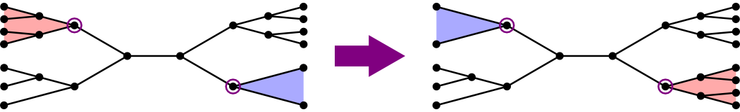
• Works well in theory, but it might be too expressive.
• Every tree has many adjacent trees.
• May not be much better than a brute force search.

The approach the text uses:

• Choose a segment instead of a node.
• Swap two subtrees, one from each end of the node.

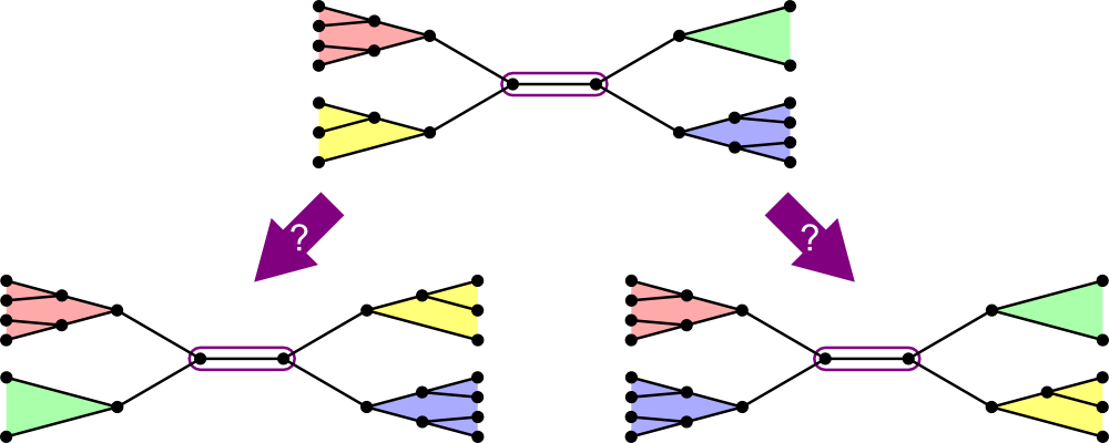
• It turns out that there are only two adjacent trees for every segment.

Where should you start the search?

• Which tree you look at first may affect which tree you end up at.
• There are two approaches often used for search problems:
  1. Heuristic best estimation.
  2. Rapid Random Restart (RRR).

Using a heuristic best estimation:

• Solve the problem using another method, then use that solution to start the search.
• Basic idea: if you can start close by your final solution, the search will be faster and more likely to succeed.

Rapid Random Restart:

• Do the search many times, each time starting from a totally random starting place.
• Don't spend a ton of time searching:
  • Take a few steps.
  • Get a good feel for how well you're doing.
  • Move on.
• Ultimately, you can further explore the path that looked the best.

For the parsimony problem, we can use the former approach:

• Solve the ancestry problem using another method (like Neighbor Joining).
• Use this tree to start the most-parsimonious-tree search.
• Might bias the results.

Branch and Bound

There is another way to shortcut the search for the most parsimonious tree.

• Branch and Bound

Notice that as a tree gets bigger, its cost will only increase.

• No segment ever has a negative cost.
• Thus if you add a segment, its cost will either go up or stay the same.
• If a subtree already costs more than some complete tree, you don't need to look any farther.
• You can exclude many trees from your search in a single step.

What you need is to enumerate all trees, in a way that you look at their subtrees too. Here's one method:

• Make an array of size (n-3).
  • Label each element i₃, i₅, i₇, etc.
• Start with a basic tree linking taxa A, B, and C.
• Run through the array like an odometer.
  • Each value tells you where to add new segments.

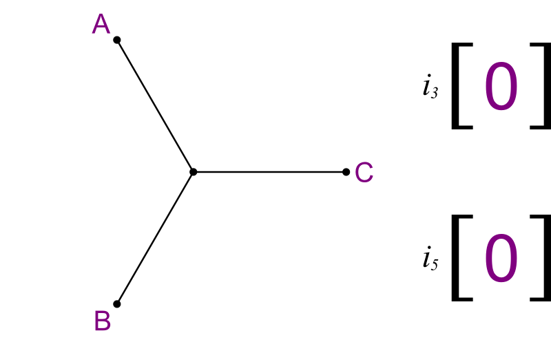
• Each element can range from 0 to its subscript.
• If an element is 0, all further ones must be 0 too.
• The number tells you which existing segment to add the next segment to.

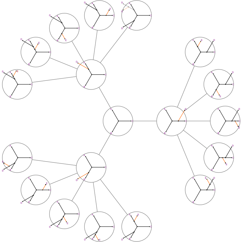
The search “branches” out.

• Start state has 3 branches, to 5, to 7...
• When you add a segment, you need to explore all of its next segments one at a time.
• But if we're beyond the cost of the best complete tree seen, we can backtrack immediately.
  • That's the “bound.”

Branch and Bound is not usually considered a heuristic.

• It will find the best tree.
• In the worst case, it will take as long as a brute force search.
• In the best case, many bounds make the search very quick.

Summary

Phylogenetic trees show the relations between many taxa.

• Rooted trees show ancestry.
• Unrooted trees just show relation.
• Rooted trees are usually preferable, but require more assumptions that may not be true.

There are usually three different approaches to reconstructing a tree:

• Distance: find the tree that accounts for estimated evolutionary distances.
• Parsimony: find the tree that requires minimum number of changes to explain the data.
• Maximum likelihood: find the tree that maximizes the likelihood of the data.

UPGMA is a distance-based method.

• Unweighted Pair Group Method using arithmetic Averages.
• Returns rooted tree from distance data.
• Successively merges clusters of taxa that are closest together.
• Distance of clusters from each other is average of component distances.
• Makes ultrametric assumption, and so often not the best choice.

Neighbor Joining is a similar distance-based method.

• Returns unrooted tree from distance data.
• Successively merges clusters of taxa that are closest together, and also isolated from others.
• Makes additive assumption, which is usually closer to true than the ultrametric assumption.
• Distance of clusters from each other is solved geometrically from component distances, assuming the data came from a tree.
• Unrooted tree can be rooted with an outgroup.

Parsimony methods find the relations that have the least amount of change.

• The small parsimony problem solves the ancestor states when a tree is already known.
• The large parsimony problem tests several trees, solving small parsimony for each of them.

Truly finding the best tree by parsimony is usually an intractable problem.

• Can use search heuristics to only test a subset of all possible trees.
• Branch and Bound can also cut the search space using a non-heuristic method.