BioMesh Project
An
All-Hex
Meshing Strategy for Bifurcation Geometries
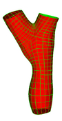
Single Bifurcation Model
|
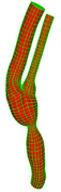
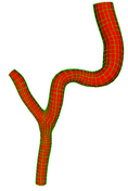
Multiple Bifurcation Model
|
 |
|
Data Source:
Prof. Francis Loth, UIC
|
Data
Source : Arizona State University
|
Introduction:
Bifurcation
is very common in all
natural flow carriers (example
arteries,
veins etc.). Most of the numerical flow simulation using
Navier-Stokes
equations require a high quality discretization of computational domain
into 2D (Triangles, Quadrilaterals or Polygons) or 3D simplexes (
tetrahedra, hexahedral,
prism, or hybrid). The selection of element shape is decided by
the solver, accuracy and resource requirements. Unstructured
tetrahedral mesh, although,
much simpler to generate, may require large number of elements to
resolve very small scale
phenomenon compared to structured or
unstructured hexahedral mesh.
In this project, we implement a robust algorithm to generate All-Hex
elements in bifurcation and tubes arbitrary shapes arising in
subject specific computational hemodynamics modelling. The
key
components of our approach are the use of a natural co-ordinate system,
derived from the solutions of Laplace's equations
that follows the
tubular vessels. We demonstrate with many different geometric models,
that a very high quality hex mesh can be
generated in a fast and accurate way.
For the following geometric models, you may download
1. Surface Triangulation
2. Tetrahedral Volume Mesh
3. Hexahedral Volume Mesh ( Level I, II and III )
Acknowledge: All the visualization have been done using
ParaView Software.
Methodology:
Table of Contents
1. Introduction
2. Procedure
3. Performance
Results
A general pipeline starting from image acquisition from various
modalities till the mesh generation for the numerical simulation is as
follows. One of the main goal of this project is to automate the
entire process with minimal human intervention.

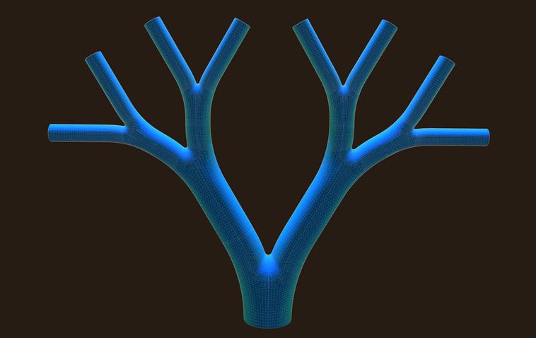
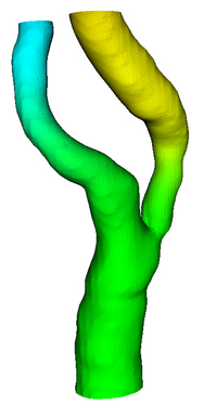
Given a general bifurcation geometry as shown below, our algorithm will
generate a high quality all hexahedral mesh in the tubular domain
satisfying two requirements:
- No two cross sections intersect.
- Each cross section is orthogonal to the vessel wall.
- Number of hexahedral elements must be small and predictable.
Fig: (I) Domain decomposition of a vascular geometry
into
six regions
(II) Each region is mapped to a canonical half cylinder
Some existing general purpose all-hex mesh algorithms
- Whisker Weaving ( Timorthy J. Tautges )
- Plastering ( Steven J. Owen )
- Medial Axis Decomposition
- Octree
All the above algorithms have been
used in varieties of applications.
Compared to a general purpose approach, our domain specific approach
has the following features.
1. Specifically designed for tubes and bifurcations,
2. Easy to
implement with reusable software
components ( > 90 % reuse)
3. Produce very high
quality mesh.
4. Number of mesh
elements and spacing can be controlled.
5. Numerically robust.
We have been using these geometries to study turbulence in human
carotid
arteries which develop atherosclerosis causing stokes. For more
details, read an article from Dr. Paul Fischer entitled "Stroke
Busters in Turbulent Blood"
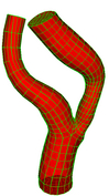
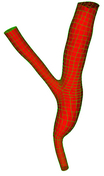
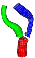
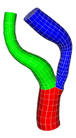
Domain Decomposition:
The fundamental problem with the bifurcation problem is related to
"Domain Decomposition". How can we divide the three vascular tubes into
three domain, each of the domain should be topologically equivalent to
a one-dimensional tube. The following pictures describe the
decomposition performed by our method.
Fig: Domain
Decomposition of vascular geometry into three tubes.
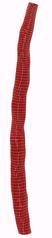
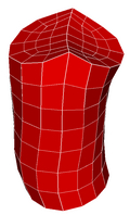
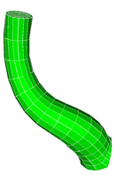
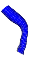
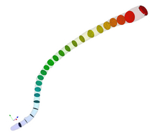
Basic Idea:
Consider an undulating tube with varying diameter. Let us solve the
Steady thermal conduction problem with the following boundary conditions
- T = Ta At the opening cap;
- T = Tb At the end cap
- On the side walls DT/DN = 0 where
N
is outward normal to the boundary surface.
Assume that Tb > Ta and now construct the isosurfaces
of
monotonically increasing sequence of temperatures Ta = a1 < a2 <
a3 .... =Tb. These isosurfaces will be non-intersecting and orthogonal
to the
wall. In other words, these isosurfaces create a natural
coordinate system.
Fig: Isosurface in an undulating
tube creates a natural coordinate system.
We want to extend this idea create all-hex volume mesh in bifurcation
geometries. In the following sections, we will explain the entire
process. For greater details, refer to our publication.
Short Description of the Procedure:
Step I: Surface Reconstruction
Let us assume that image segmentation and registration is already
performed and that produces a noisy point cloud. The first
step in the generation of the volume mesh is to produce a high quality
surface representation. Among the various schemes, Implicit Surface
Reconstruction using Radial Basis Functions ( RBF) and Surface
Reconstruction using Delaunay Triangulation (Dey, Ameta etc.) are the
most popular choices. For detail descriptions, refer to SRPC.
The following pictures shows surface reconstruction using RBF and
Delaunay Triangulation (DT). Perhaps the biggest advantage of RBF
is
in
filling gaps in an undersampled dataset. As shown in the
following picture II, RBF can also fill a gap in some unwanted regions.
This
necessitates visualization, manual clipping and therefore, hinders full
automation.
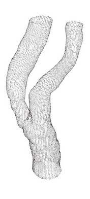
Input Point Cloud
|
RBF
Surface
|
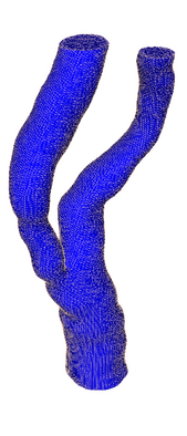
Delaunay Surface
|
Fig: Surface
Reconstruction using Point Cloud
The following table shows that system of linear equations arising from
thin plate RBF are ill conditioned which become worse as the number of
sample points increases.
|
Matrix Size |
Condition
Number |
239x239
|
2.5645 x 10^5
|
447x447
|
1.1683 x 10^6
|
1256x1256
|
1.5976 x 10^7
|
Surface reconstruction using DT is extremely fast
and provably correct. Perhaps the only disadvantage of this
approach comes while handling undersampled dataset. However, it is
possible to
detect undersampling in the dataset while creating DT, therefore,
surface repair tools can be applied on the undersampled regions.
At a final step in surface reconstruction, mesh optimization
schemes 1) Edge Flipping 2) Non-shrinking surface
smoother (Taubin Smoothing, Mean Curvature flow, or Implicit Fairing
) are applied to remove additional noise in the dataset. For
details, refer to
SurfSmooth
Step
II: Classify Surface Vertices:
The output of step one is a
clean, noise free, smooth 2D
manifold surface triangulation. In order to solve the Laplace equations
(
described in the next section ), we have to
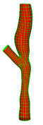
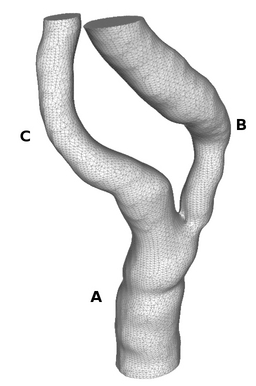
classify surface vertices into three categories i.e. surface (1) ,
inflow (2) , and
outflow (3 & 4) ( Assuming that in the following picture, the
inflow is at the bottom and two branches are
outflow). At least one vertex must be classified as
inflow and two vertices as outflow.
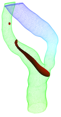
In order to automate identification of inflow and outflow vertices from
the surface model, a Reeb graph (or Medial Axis) is constructed which
has the shape of "Y". ( Reeb graphs is very simple to construct
compared to Medial Axis). The end point of the hand is "inflow" and the
fork ends are "outflow" vertices.
Surface Model
|
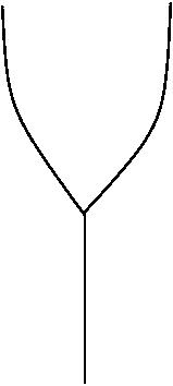
Reeb
Graph
|
Fig: (I) Surface Triangulation (II) Identifying end
points with approximate MD.
Step 3:
Tetrahedral Volume Mesh Generation
Using the surface triangulation as
constraint, generate a tetrahedral
volume mesh. (Many Delaunay triangulation based software may insert new
vertices on the surface). Since the
quality of the volume mesh
is not critical for the final hex mesh generation, therefore, any
suitable
tetrahedral mesh generation ( of course without slivers ) can be
used.
In our case, we used SolidMesh software based on
Advancing
Front Technique (AFT) to
obtain the
tetrahedral volume mesh.
If the surface is not properly sampled or has holes, we use RBF
Implicit surface reconstruction algorithm to create a smooth 2D
manifold surface. In this
procedure, too many triangles are generated
that are needed to solve the heat conduction problems and subsequently
mesh generation. Therefore, a
coarser grid is obtained by finding "Independent Set" from the
mesh graph. "Topological Noise" is the biggest problem in the
surface reconstruction through implicit polygonization. The
holes can be identified by calculating Euler Characteristic of the
surface. At present, we don't have robust implementation to
remove the "Topological Noise", therefore, we experimented with
different spacing in MC and were able to get zero genus surfaces.
Step 4: Solving
Heat Conduction Problems:
As described in the paper the central
theme of our approach is to
create
a natural co-ordinate systems by solving three different Laplace
Equations with the following Dirichlet and Neumann
Boundary Conditions. For this purpose, standard Finite Element
Formulation ( FEM) is used. The symmetric, positive definite
system of linear equations arising from FEM is solved using
Preconditioned Conjugate Gradient method. ( We used Matrix Template
Library MTL for Matrix objects and Iterative Template Library ITL for
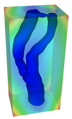
PCG) . The color plots of the temperature
distribution are shown in the following pictures.
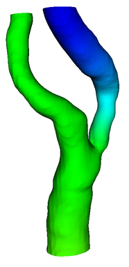
Branch
A: Insulated
Branch B: -Ta
Branch C: 1-Ta
|
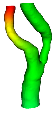
Branch
A: 1-Tb
Branch
B: Insulated
Branch
C: -Tb
|
Branch
A: -Tc
Branch
B: 1-Tc
Branch
C: Insulated
|
Fig: Temperature distribution
Observe that there is rotational symmetry in the boundary conditions,
which can be exploited to reduce the code size. How should we select
the Dirichlet Boundary condition values ? We can choose any
two values, but any arbitary values may not give a same value on
the insulated cap for all the three cases ( It is must and the reason
will be explained later). Therefore, for each case, we solve
Laplace solver twice in order to ensure that the end cap of each
insulated boundary is maintained at the same value.
For each case, in the first run, we specify Dirichlet values 0
and 1 at two ends. This will create some temperature ( let us say
alpha) at the cap of insulated boundary. In the second run,
Dirichlet Values are shifted by alpha, so that the temperature at
the center of the insulated end cap becomes zero.
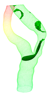
The Isosurface emanating from the center of insulated caps are called
"Principal Isosurfaces".
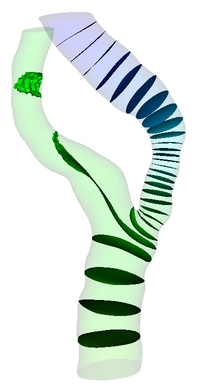
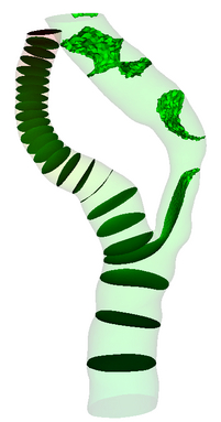
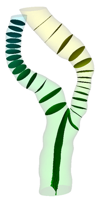
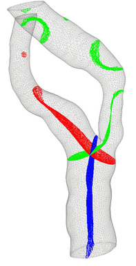
Step 5:
Constructing Primary Chips:
Obtain the three iso-surfaces at T =
0 from each solution. Ideally,
with the exact arithmetic, we should get a smooth surface from the
centre of insulated cap and right upto the end near the
bifurcation, but as
shown in
the pictures, iso-surface away from the centre are jig jagged and
sometimes there may be pockets of
isolation. This behaviour is because of finite numerical
precision, but our region of importance (ROI) is
the "Bifurcation Centre", where all three iso-surface are smooth.
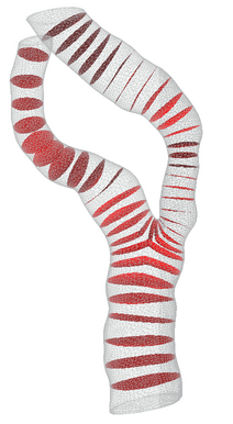
Fig:
Isosurfaces from the solution of heat conduction problems.
IsoSurface A
|
IsoSurface B
|
IsoSurface C
|
Intersection of IsoSurfaces
|
Fig: Creating principal chips with principal isosurfaces which emanates
from the insulated BC branch.
Use implicit surface cutter to remove the part of the surface that is
not required.
Zoomed Picture
|
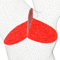
Primary Chips
|
Topology of A Chip
|
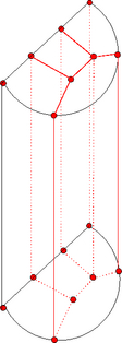
|
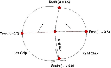
Fig: (I) A zoomed picture of Principal Chips ( A and B).
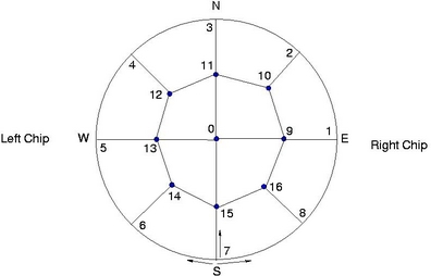
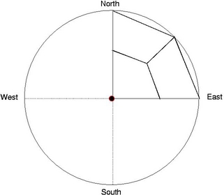
(II) Topology of each chip. (III) A half cylinder
"South Vertex" of the primary
chip acts as a reference point for
the
proper orientation of the subsequent chips. Three curves (left, right,
and Interface boundary) are parameterized with
south (u = 0.0) and north (u= 1.0). East, West and Center vertices are
then determined at u = 0.5 along these curves.
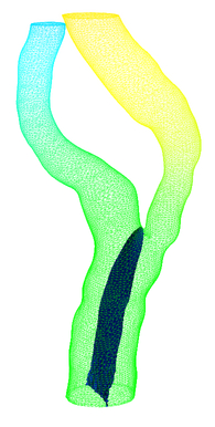
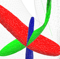
Step 6:
Constructing Split and Simple Chips:
As we move away from the bifurcation
region, the angle between the left
and right chip decreases ( as shown in the zoomed picture below) . When
the angle between right and left chip
become less than 10 degrees, ordinary chips
are constructed from the isosurface in the branch.
Chips in Artery
|
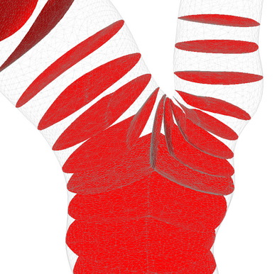
Zoomed Region Near the Bifurcation
|
Note: Simple chips near the end caps may be distorted or cut
depending upon the geometry and boundary conditions applied on selected
vertices. There are two options (1)
Reject the chips that are not proper (2) Start with an
artificially extended branch and then discard all the chips in the
extended branch.
Pseudo-codes for constructing Split and Simple chips are given below.
Note that Isosurface extraction and implicit surface cutter are the
only two software modules that are required to create chips. Also note
that, isosurface extraction from tetrahedra mesh will be called large
number of times and it is the most expensive compared to other calls,
therefore, any optimization can have significant improvement in the
efficiency of the algorithm.
Algorithm: ConstructSplitChip ( tetmesh, branchID,
isoVal,
center0)
//********************************************************************************
// Input Parameters:
// branchID : The branch in which which Split chips
are created.
// IsoVal : Temperature
value for which the right surface of the chip is constructed.
//
The left side depends on the location of the right ( because of
alignment).
// center0 : Approximate
center of the previously generated chip.
//*********************************************************************************
bA = ( branchID+0)%3
bB = ( branchID+1)%3
bC = ( branchID+2)%3
// Search for right half of the chip separated by distance "width"
while(1) {
rightmesh = getSurface( tetmesh, isoval, bA)
cutmesh = getCutSurface( rightmesh, 0.0, bC) //
Implicit Cut the surface
interface =
getInterface(cutmesh)
// Extract the Cut boundary contour
center1 = getCenter(
cutmesh)
// Get the center of interface contour
if( dist( center0, center1) > width) break;
}
discard( rightmesh,
-1)
// Remove the left portion of the righmesh.
addInterface( chip,
interface)
// Add the interface
addSurface( chip, rightmesh,
1) //
Remaining mesh constitutes right half of the chip.
// Create left half of the chip, such that interface align together.
isovalB = getIsoValue( center1,
bB)
leftmesh = getSurface( tetmesh, isoValB, bB)
cutmesh = getCutSurface( leftmesh, 0.0, bC)
discard( leftmesh,
1)
// Remove the right side of the leftmesh.
addSurface( chip, leftmesh,
-1) // Remaining
mesh constitutes left half of the chip.
Algorithm : ConstructSimpleChip(
tetmesh, branchID, isoVal, center0)
trimesh = getSurface( tetmesh, isoVal, branchID)
addSurface( chip, trimesh)
Step 7:
Apply Mesh Templates on each Chip:
Each Chip can be divided into four
quadrants and user defined mesh
templates as shown below can be applied on each chip. Vertices are
always projected on the chip surface
constructed by the isosurface. With increasing level of subdivisions,
better approximation of the outer surface is obtained.
Level-0 Mesh Template
|
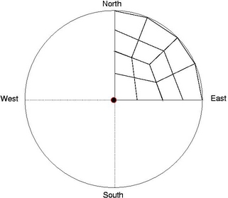
Level-I Mesh Template
|
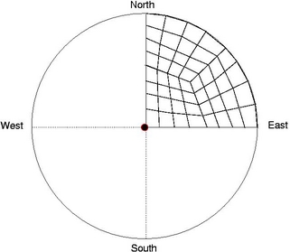
Level-II Mesh Template
|
Fig: Examples of Mesh Templates.
Step 8:
Smoothing QuadMesh on each Chip:
Isosurface generate
triangulated surface which acts as a
background mesh on which the quadrilateral mesh is superimposed. The
quality of quadrilateral mesh depends on the
node distribution on the background mesh. As the number of levels
increases, two or more points
may project on the same node of the background mesh which will result
in zero edge length of some
quadrilaterals. Therefore, it is essential to apply smoothing,
after mesh template is
applied. Experiments shows
that, 4-5 steps of Taubin's smoothingis sufficient to get very good
quadrilateral mesh.
Step 9: Create
Volume Mesh:
After consistently orienting each
chip with respect to the
primary chip, volume mesh is constructed using quad-mesh from two
consecutive chips. As the number of chips and
quad-mesh is deterministic, total number of hex-elements is also known.
In order to ensure that each hex is positive, Jacobian at each eight
nodes is checked.
Step
10: Apply Volume Mesh Optimization and Obtain Quality
Statistics.
The quality of the volume mesh may be
further improved by using
standalone Mesh Optimization Tools ( such as Mesquite). Volume
mesh, however, can not be improved beyond a limit unless the
surface mesh is also improved and/or topological flipping operations
are carried
out. (At present, we have not implemented these optimization)
Out of many quality measures, we measure only few to ensure that the
correctness of the final volume mesh.
1. MinMax Volume.
2. MinMax Aspect Ratio
3. Worst Condition Number.
Performance Results:
Module
|
Time ( in
seconds)
|
Vertex
Classification
|
|
Heat
Conduction Problems
|
|
Chips
Construction
1. Primary Chips
2. Split Chips
3. Simple Chips
|
|
Mesh
Templates
1. Level I
2. Level II
3. Level III
|
|
Mesh
Smoothing
|
|
Volume
Meshing
|
|
Volume Mesh
Optimization
|
|
Quality
Checks
|
|
Software:
Presently, the source code is not
ready for public distribution.
Please contact Dr. Paul Fischer (E-mail: paul@mcs.anl.gov)
for further information.
File Format:
All the files are in ASCII and the data format is as follows. For order
of connection, refer to MeshDatabase
#Nodes Number of Nodes
x1 y1 z1
x2 y2 z1
.
.
.
xn yn zn
#Triangles Number of Triangle
v11 v12 v13
v21 v22 v23
.
.
.
vn1 vn2 vn3
#Quads Number of Quads
v11 v12 v13 v14
v21 v22 v23 v24
.
.
.
vn1 vn2 vn3 vn4
#Hex Number of Hex
v11 ... v18
v21 ... v28
.
.
.
vn1
...
vn8
Note: All vertex index starts from 0 ( not 1 as in FORTRAN) and
are contiguous.
Presentation:
14th IMR Conference, San Diego Presentation 13th Sep, 2005 Download Presentation.
(The paper is also available
in the Proceedings of the 14th International Meshing
Roundtable )
Publications:
- An All-Hex Meshing Strategy for Bifurcation Geometries in
Vascular Flow Simulation
Chaman Singh Verma, Paul F.
Fischer, Seung E. Lee, F. Loth
14th
International Meshing Roundtable Conference-11-14 Sep, 2005, San-Deigo,
California
Download
Paper
- Re-engineering Legacy Code with Design Patterns: A Case Study in
Mesh Generation Software
Contact :
Paul Fischer
Mathematics and Computer Science Division
Argonne National Lab
fischer@mcs.anl.gov
|
Francis Loth
UIC College of Engineering,
FLoth@uic.edu
|
Chaman Singh
Verma
Mathematics and Computer Science Division
Argonne National Lab.
csverma@mcs.anl.gov
|
|
Last Modified: Wed Sep 31
17:03:06 CDT 2006