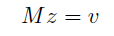
Photometric
Stereo
Chaman Singh Verma and Mon-Ju Wu
|
|
|
 |
 |
 |
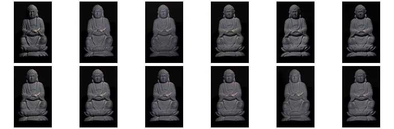
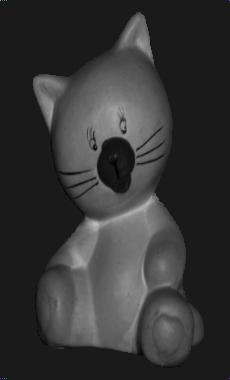
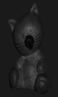
Original
Image
|
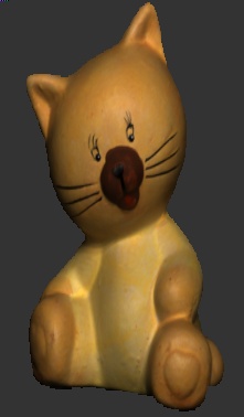
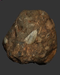
Albedo
|
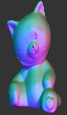
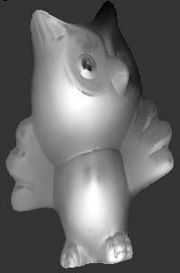
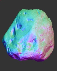
Normal Map
|
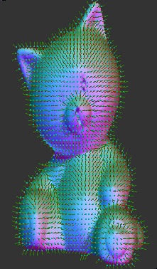
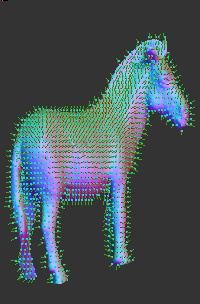
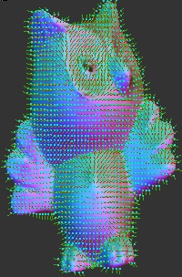
Normal
Vectors
|
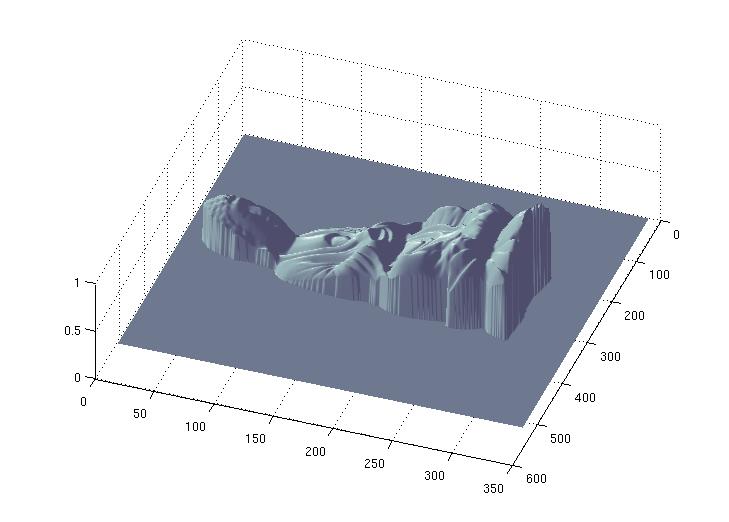
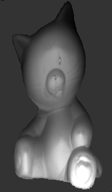
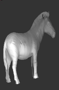
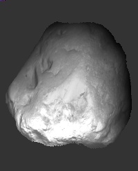
Height Map
|
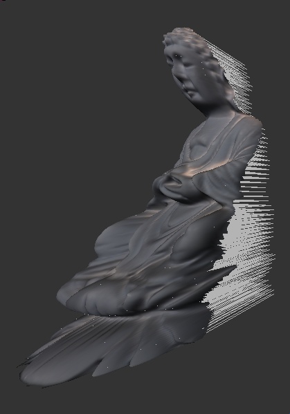
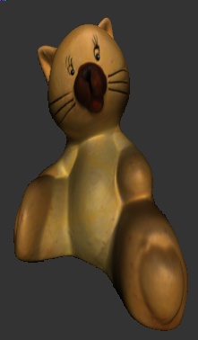
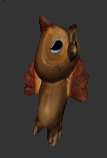
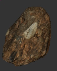
3D Rendering
|
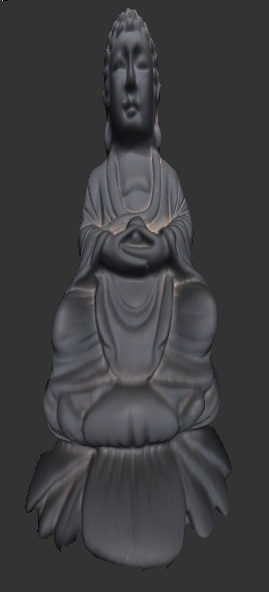
Introduction:
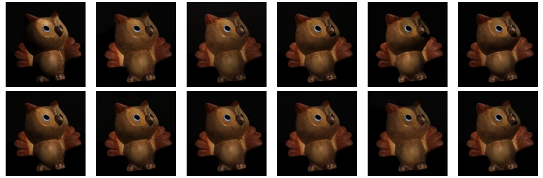
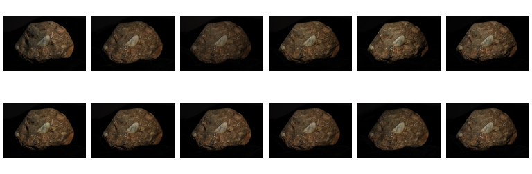
Photometric stereo is a technique to estimate depth and surface
orientation from images of the same view taken from different
directions. Theoretically, only three directions are sufficient to
obtain normals, but to minimize noises inherent in the process, more
than minimum number is often required for realistic images. This
method, however has some limitations (1) Light source must be far from
the objects (2) Specular or dark spots in the regions don't give
satisfactory results (3) shadows must be masked to avoid for valid 3D
surface reconstruction.
There are two coordinate systems (1) Image based coordinate system in
which upper lower is the origin and downward "y" is positive (2) Right
hand world coordinate system in which x goes from left to right, y from
bottom to top and "z" from back to front. Throughout the project, we shall
stick to right hand world coordinate system.
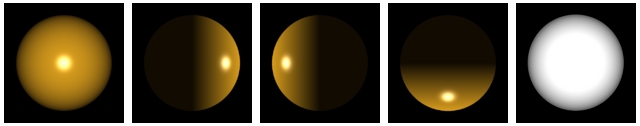
Light Calibration
The
first step in the calculations of normal map is to calibrate light
source i.e estimate the light direction. One way to do this is to use
chrome ball on which the brightest spot is used to identify the
direction of the light.
 |
 |
|
Synthetic data generated using OpenGL to verify light caliberation |
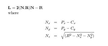
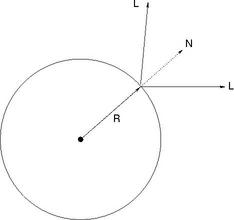
Where R is the reflection direction taken as [0,0,1]. Here [Px,Py] is
the location of brighest point on the chrome image and [Cx,Cy] is the
center of the chrome in image space which can be estimated by the
maskimage/
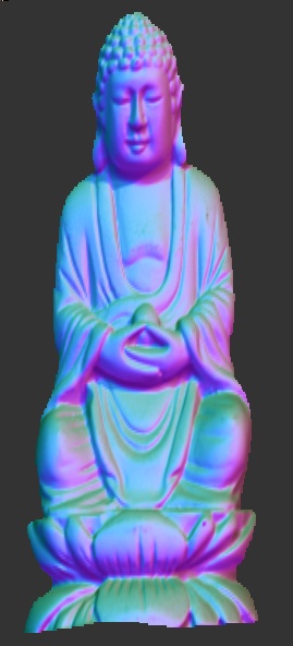
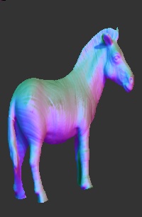
Normal Map Generation :
For lambertain surfaces, intentity at any point on the surface can be
given as
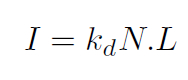
Where N is the normal at the surface point and L is the reflected light
direction. In order to determine N, we need at least three light source
which
are not in the same plane. Therefore the above equations can be written
as
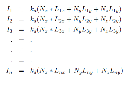
Now let us denote
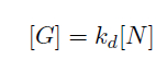
So for n > 3, we can solve the equations with least square methods as
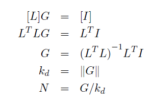
Therefore, we can retrieve both normal and albedo map per pixel, if the
pixel receives light from at least one source. In practice, there are
many pixels in the region where light intensity from the sources is
very low, so we need to skips those pixels for calculations. Matlab
implementation of the this code is very straightforward.
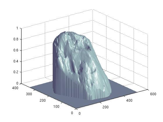
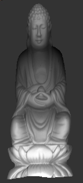
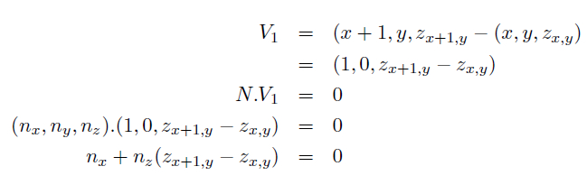
Depth Map Generation:
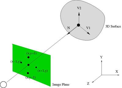
The Normal at surface must be orthogonal to the vector V1 gives:
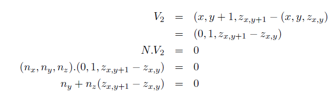
The normal at surface must be orthogonal to the vector V2 gives
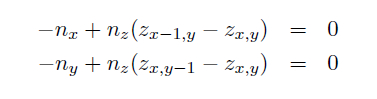
Boundary conditions or pixels where either (nx,ny,nz) values are not
available must be taken into consideration. At those pixels, instead of
taking forward step for depth calculation we take forward direction
that modifies the above equations as
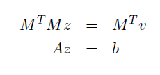
This generate a sparse matrix of (2*numPixels, numPixels) ( where
numPixels are the pixels in the masked region and not the entire
region) where each row contains only two entries. This overdetermined
system of liner equations is solved by least square method of conjugate
gradient method by making equation symmetric and positive definate.
or equivalent system:
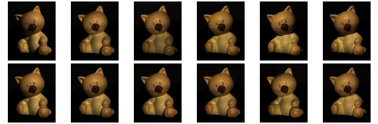
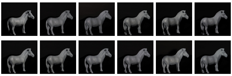
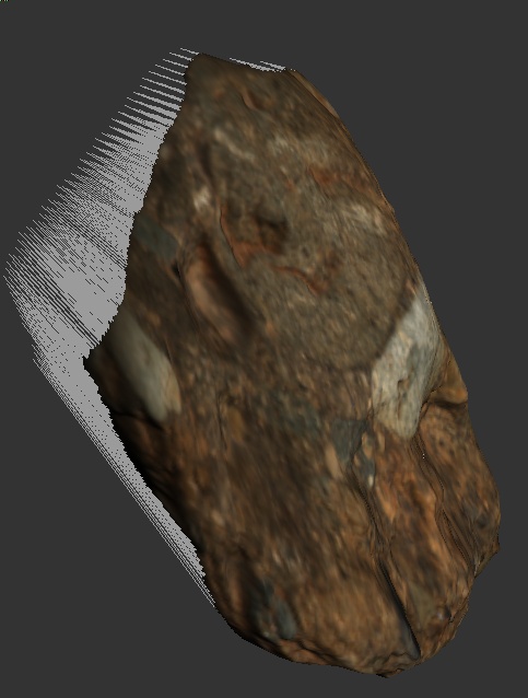
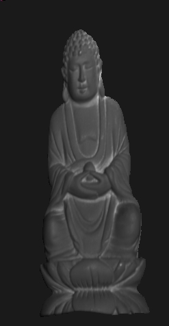
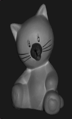
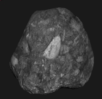
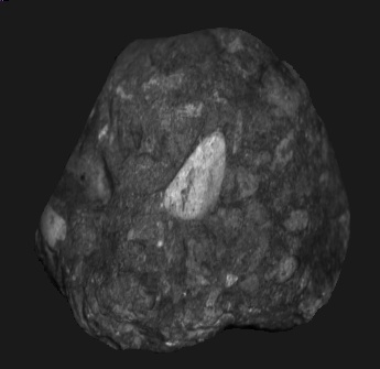
Results:
The following dataset were provided by Dr. Li Zhang for this class
project.
|

|

|
Red Albedo
|
Green Albedo
|
Blue Albedo
|
|
|
|
Red Albedo
|
Green Albedo
|
Blue Albedo
|
|
|
|
|
|
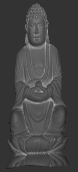
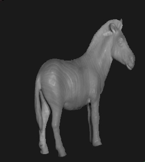
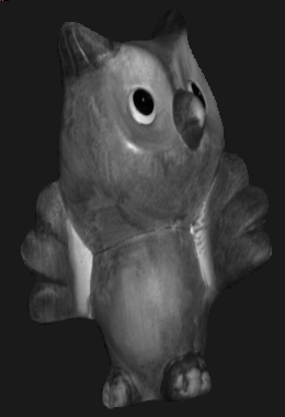
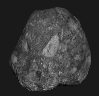
Original
Image
|
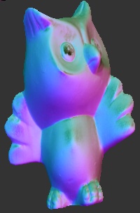
Normal Map
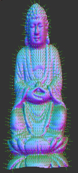
|
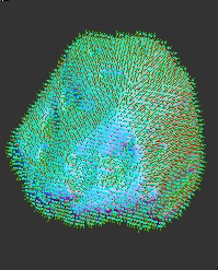
Normal
Vectors
|
HeightMap
|
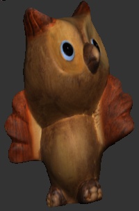
3D Rendering
|
|
|
|
Red Albedo
|
Green Albedo
|
Blue Albedo
|
|
|
|
|
|
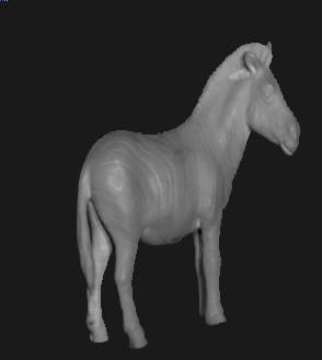
Original
|
Normal field
|
Normal
Vectors
|
Height Map
|
3D Rendering
|
|
|
|
Red Albedo
|
Green Albedo
|
Blue Albedo
|
|
|
|
|
|
Original
|
Normal map
|
Normal
vectors
|
Height Map
|
3D Rendering
|
|
|
|
Red Albedo
|
Green Albedo
|
Blue Albedo
|
|
|
|
|
|
Original
|
Normal Map
|
Normal
Vectors
|
Height Map
|
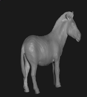
3D Rendering
|
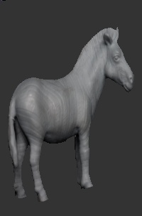
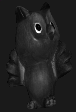
Discussions and
Conclusions
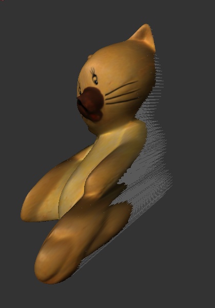
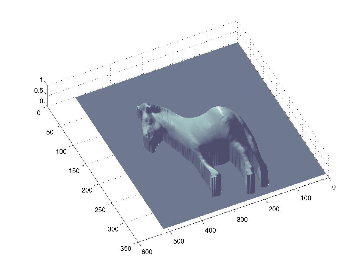
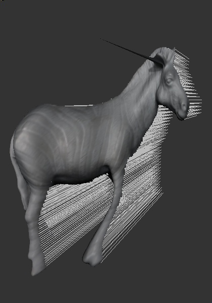
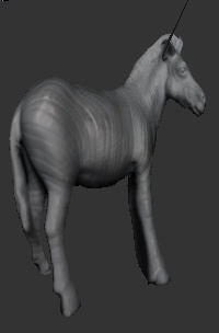
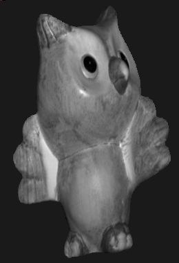
- It seems that present method (which
is quite naive) is poor in
handling dark spots in the image. Both owl's eyes and horse ears we can
observe the spiked artifacts.
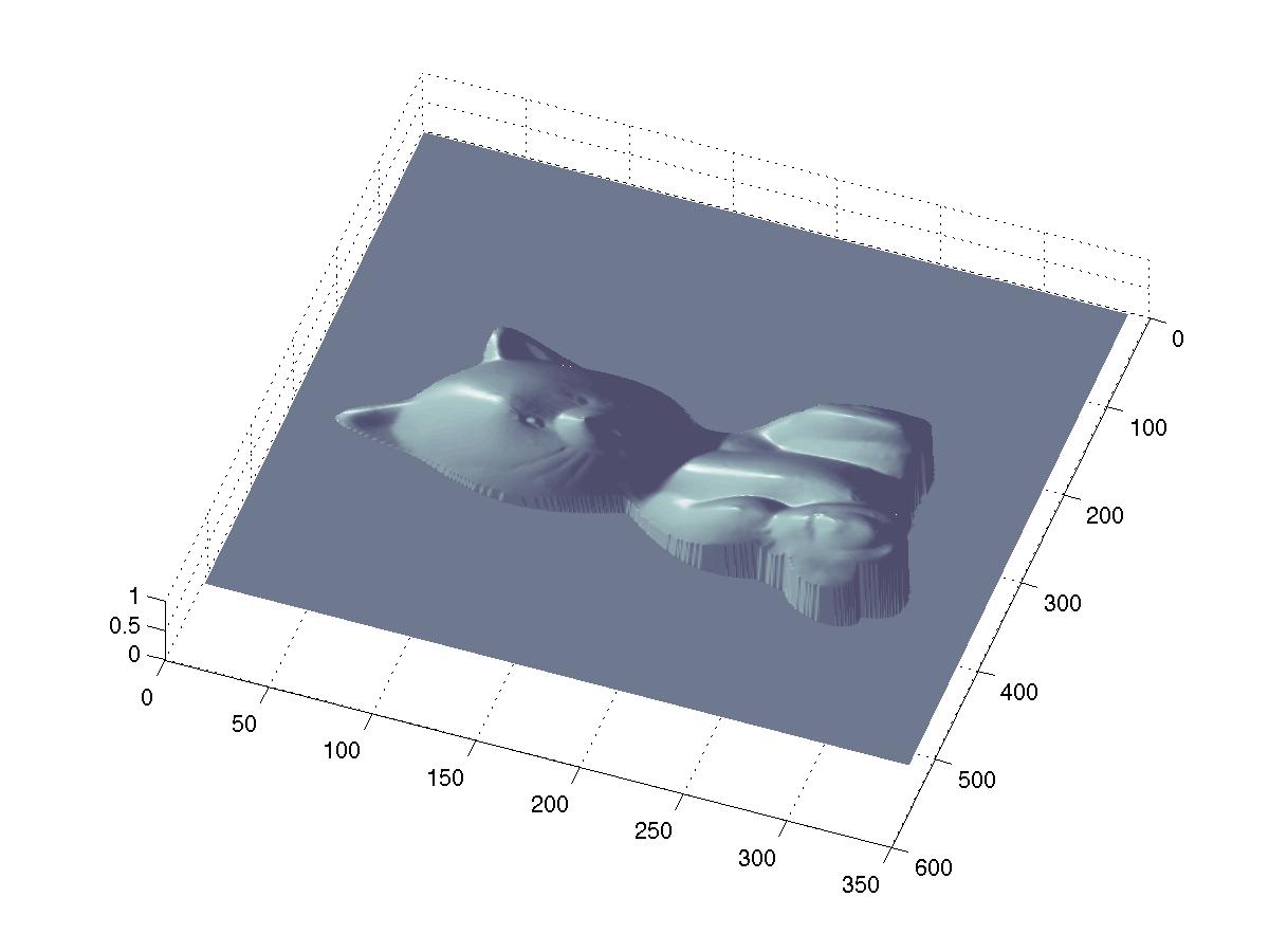
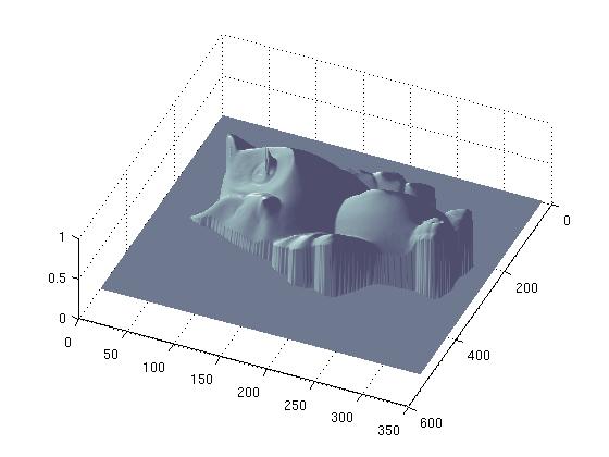
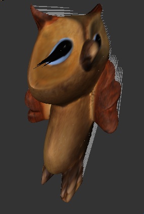
- Although the owl's depth map looks
quite reasonable, the 3D
rendering is not impressive. There is definately distortion because of
scaling effect.
- Since the depth map calculations are
valid for arbitrary scaling,
the "Z' values are also scaled. Perhaps the Z scaling could be
calculated by matching normals from the 3D reconstructed model. ( But
we didn't carry out this exercise in this study).
Software and User's Guide
The entire software is written in Matlab because it requires some
sparse linear system solvers and it was quick to implement it. There
are four main modules in this software
- Stereo.m
: Main Driver routine
- CalibrateLight.m
: Function to calibrate light with the given chrome ball.
- NormalMap.m
: Generate Normal Map given Light Directions
- DepthMap.m
: Generate Depth Map given Normal Map
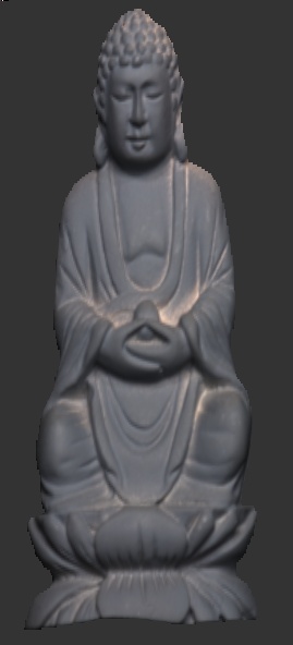
The use of the software in simple, just write on Matlab command prompt
z = Stereo( directory,
dataset, numImages)
Where "directory" folder contains (1) A folder named dataset
which contains all the images (2) "chrome" directory containing chrome
ball information, which is used to caliberating light directions.
The third argument "numImages" is the number of images in the
dataset directory. Example
z = Stereo( './DataSet', 'buddha', 12 );
The image are generated using libQglViewer library which is based
on OpenGL and Qt. The source code of viewer is ( not user friendly
right now ). main.cpp simpleViewer.h
simpleViewer.cpp
Group Work Contribution
Initially Mon-Ju did the light
caliberation part and myself ( Chaman
Singh ) developed the NormalMap.m and DepthMap.m codes in Matlab. But
we faced lots of troubles in getting the right results. So after we
decided that Mon-Ju should write a new Matlab with a fresh outlook and
not taking any feedback from our previously developed code, so that we
could debug and understand some missing points. We took lots of help
from Joel, Adrian and Dr. Zhang for many issues in developing the final
code. Although the entire project looked very simple in the beginning,
it tooks lots of time in figuring out the problems and all of them were
related to mixing coordinate systems from the paper, our own
interpretation and openGL coordinate system. Perhaps the biggest
lesson, we learned in this project is to choose one coordinate system
and "remain consistent" with it thoughout. Although the crux of the
code ( DepthMap.m) was written by Mon-Ju, it was significantly
modularised and cleaned by me. All the final results, visualization and
document were contributed by me.