|
|
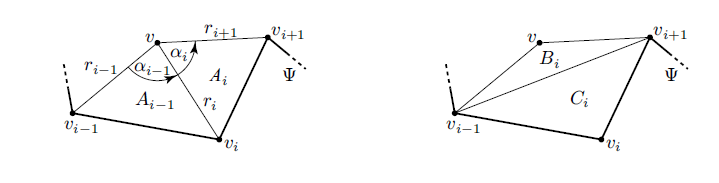
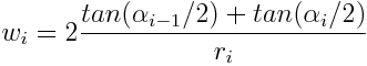
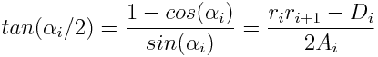
Mean Value Coordinates
2. Harmonic Coordinates (HC)
For highly concave polygonal shapes, the MVC could be negative.
Smoother and positive coordinates are generated
by solving Laplace equation for
each corner of the cage. There are theoretical results based on minmax
principles which guarantees that the values inside the domain are at
least C2 continuous.
Except for very simple geometries,
the
above equation has no closed form solution, therefore, it must
be solved by some numerical methods. Both direct solvers such as
SuperLU
or indirect iterative methods could be used. Since
this equation is symmetric and positive definite, iterative methods
such as Jacobi or Conjugent Gradient (CG) methods have very nice
convergence
properties. Jacobi method, is although simplest to implement, has
terrible convergence behavior, therefore we have used Preconditioned
Conjugate Gradient (PCG) method (with Incomplete
LU factorization as preconditioner).
First of all, in order to solve the above equation, the interior domain
must be discretized. In 2D, we used Jonathan
Shewchuk's
Triangle Software. For example,
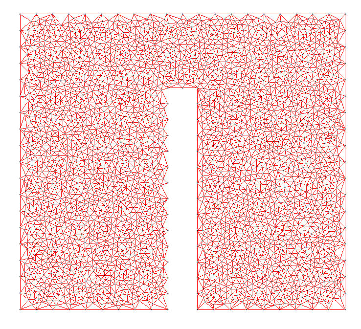
In order to get smooth results, the cage
boundary may also need fine discretization. Once the domain is
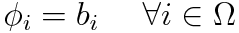
appropriately discretized, we have to set proper boundary conditions as
follows:
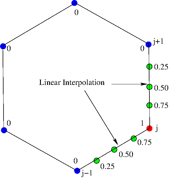
As shown in the above picture, if we
want to solve the Laplace equation
for corner vertex "j",
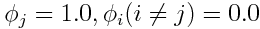
is set. The values between (j,
j+1) and (j, j-1) are linearly interpolated. Now we are ready for
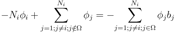
the iterative solver:
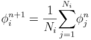
Which is simple averaging scheme around
the neighbor of each vertex. This scheme, although extremely simple as
two drawbacks (1) It starts with good convergence towards the final
solution, but as the iteration count increases, the convergence starts
crawling and it take many iteration before acceptable tolerance value
is reached (2) It is grid resolution dependent: when the grid size
increases, the convergence becomes slower.Except for some tiny grid
size, this method is unacceptable. Multigrid methods solve this
problem, but
they need complex data structures which I have not used in this
work. Instead, we solve this problem using Krylov subspace
method, which have better
convergence properties.
Standard Conjugent gradient works only
for
symmetric and positive definite matrices. With slight
modifications, the Laplace equation can be made symmetric. Laplace
equation is always positive definite:
I used ITL library (
included in MTL4 library to solve the above equations. Some
experimental results are shown in the following table ( There are lots
of scope for optimization, which is important for models with large
number of
cage points).
Laplace
Solver
|
Time(in
Seconds)
per cage point
|
Simple Jacobi
|
424
|
CG ( No Preconditioner)
|
6.725
|
CG( Diagonal
Preconditioner)
|
6.095
|
CG( ILU(0) Preconditioner)
|
5.450
|
These results were obtained on Quad-Core, Intel processor with 4GB RAM
running Ubuntu 11.04. With this experiment, we can draw some
conclusions:
- CG methods have far superior ( reduced ) time complexity.
- For this class of problem ( Laplacian ), the preconditioners did
not improve the results, Therefore, standard CG method is preferable
because of its lower space complexity.
|
|
Harmonic Coordinates
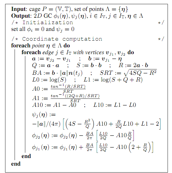
3. Green Coordinates:
Green coordinates have shape
preservation properties and like MVC, they have closed formed solution.
The exact derivation is lengthy and matematical, the pseudo code
given by Lipamn etc. is pretty straightforward to
implement. The following pseudo code is direct cut and paste from the
author's paper.
The only thing, that have to remember is
that the above formulation assume that cage coordinates are is in
clockwise direction.
Also
it
should
be
noted
that
in
the
above
code
only

needs to be normalized ( and
it is not done in the
code) and not the

.
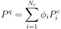
Once both coordinates have been calculated, the XY coordinate of any
point with respect to the deformed cage is given by
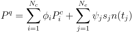
Where S(j) = length of deformed jth cage
segment/original length of the jth cage segment and n(tj) is the
outward normal to the jth cage segment. One interesting thing in
this equation is that we are adding point ( 1st expression ) with the
vector ( 2nd term), which I don't understand, therefore, I have taken
these expressions for granted.
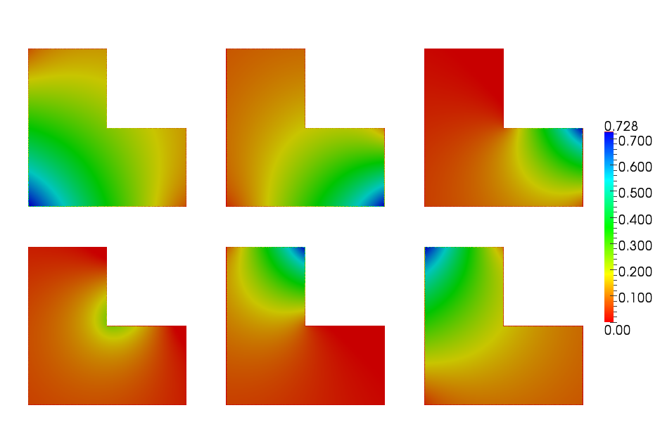
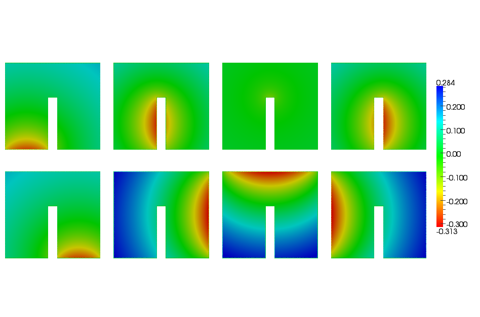
Green Coordinates's
values at each cage corners.
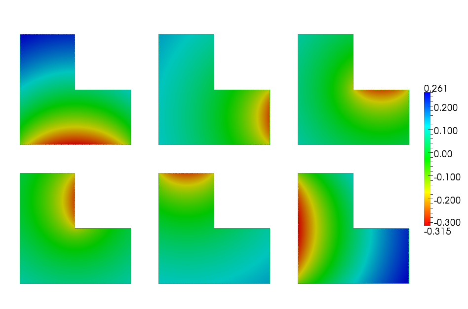
Green Coordinate's
values at each cage corners.
Comparing Time complexities:
Intuitively, both MVC and GC must be faster than HC because of the
closed form expressions and GC must be slower than MVC as it involve
many complex mathmatical expressions including exp, atan, and
log. Here is one experimental results which will give some fair
idea about time complexities of each method.
For this experiment, sampling was done on 11000 points with 4 node
rectangular cage.
Mean Value Coordinates
|
~0.1730 seconds
|
Green Coordinates
|
~0.1874 seconds
|
Harmonic Coordinates
|
~24.0 seconds
|
These results are somewhat difficult to compare with DeRose and
Meyer's paper, in which they report that HC are faster than MVC. In
fact, the timing for HC in their paper for 15362 object points in 30
second and in our
case, it is 24 seconds for 11000 points, but their timings for MVC is
113 seconds, and in our case it is 0.1730 seconds, therefore, some more
investigations are
needed to have fair evaluation of these methods. Unlike DeRose's
paper, I did not perform any
sparsification. (Or may be that MVC are harder for 3D
cages, which I did not try).
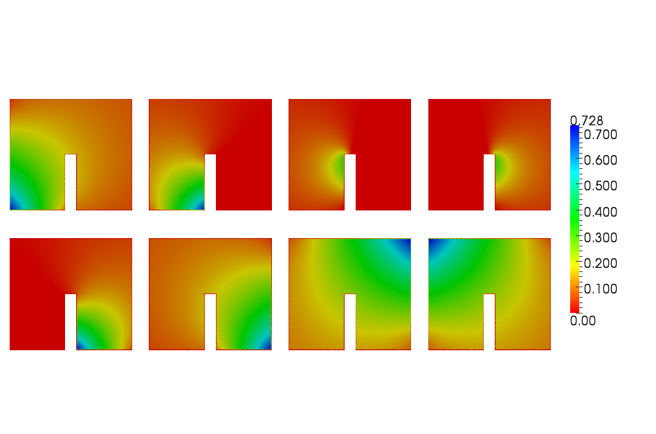
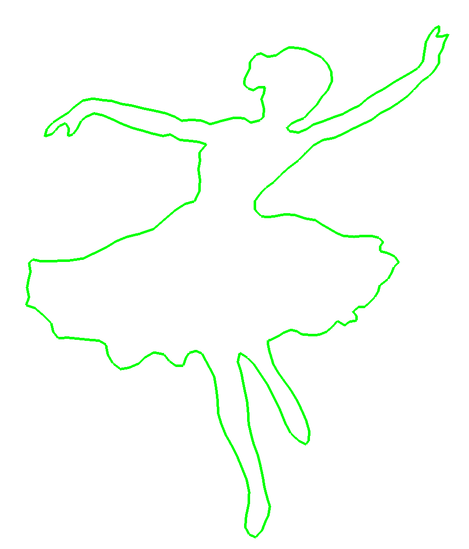
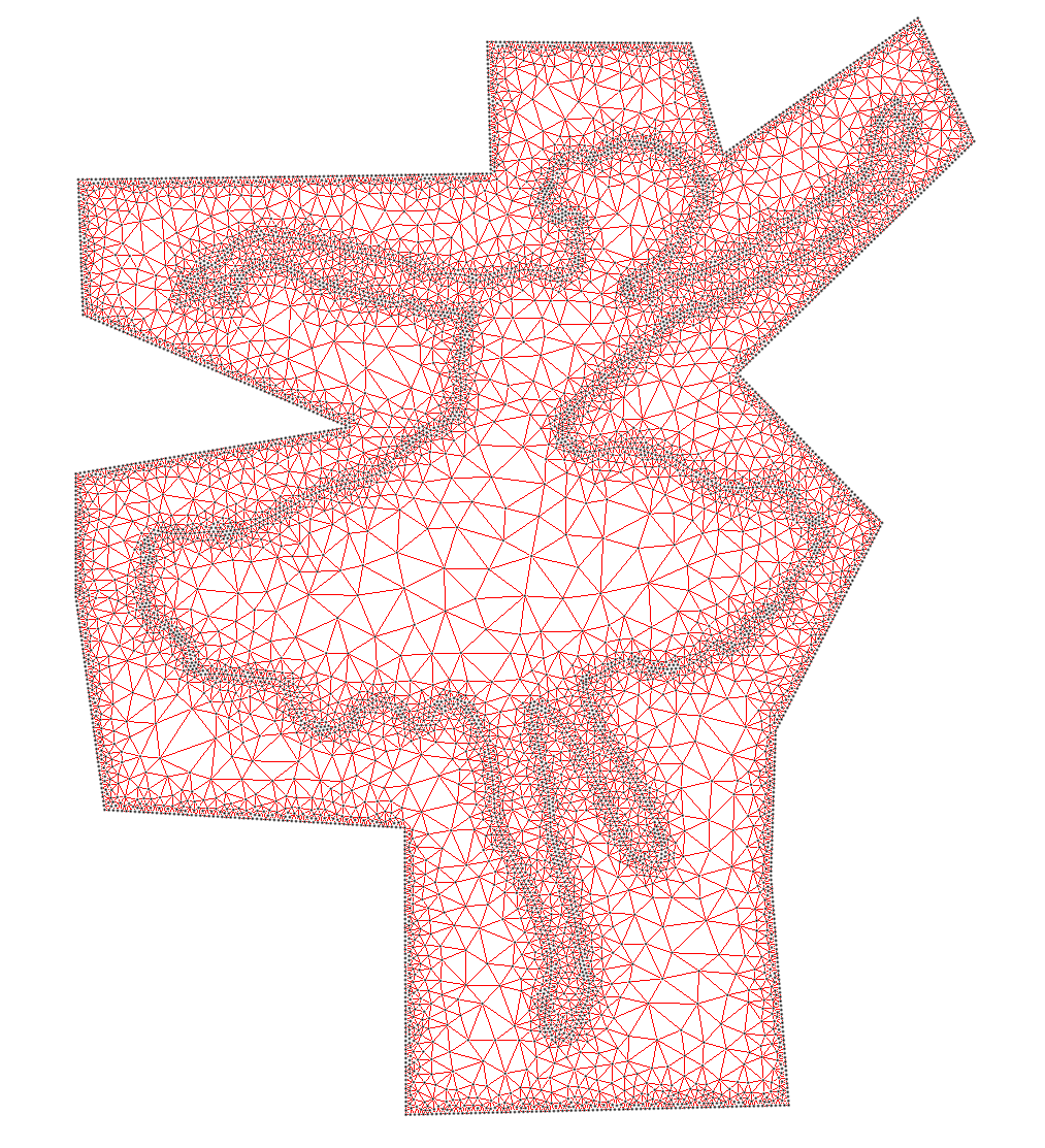
Results:
|
|
Experimental
data
and
triangulation
for
Harmonic
Field
Calculation
(
11000
points)
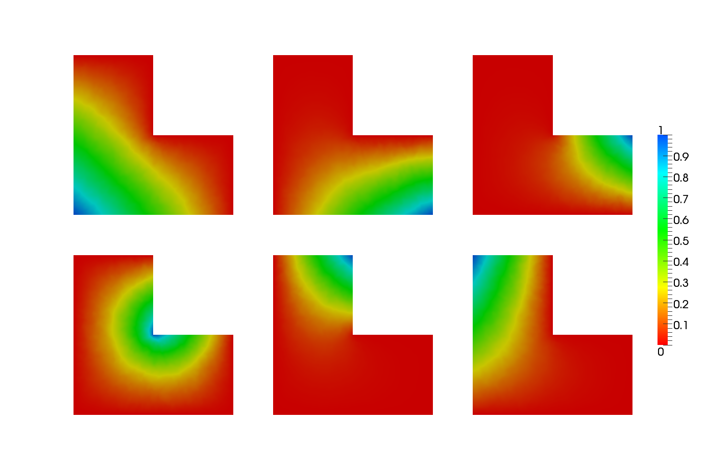
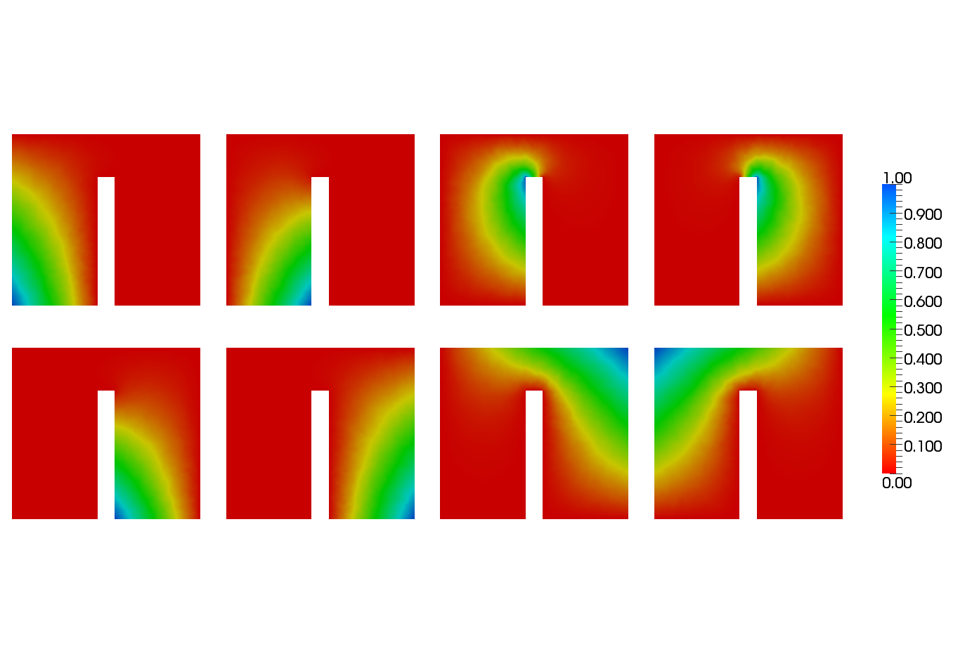
Visual evaluation : (A) Mean Value
Coordinates (B) Greens Coordinates (C) Harmonic Coordinates
Visual evaluation : (A) Mean Value
Coordinates (B) Greens Coordinates (C) Harmonic Coordinates
External Software used:
- MTL4 library for
sparse matrix storage and ITL for conjugate gradient solvers.
- Jonathan Shewchuk's "Triangle"
software for Delaunay triangulation.
- Yaron Lipman
provided Matlab code for the verification purpose.
Source Code C++
Mesh.h
Mesh.cc
GeneralizedBaryCentric.h
GeneralizedBaryCentric.cpp
( At present, the codes are not packeged properly, but fair enough for
integration).
References:
- Mean Value Coordinates:
Michael
Floater
- Harmonic Coordinates: Tony
DeRose,
Mark
Meyer
- Harmonic Coordinates for
Character Articulation: Pushkar Joshi, Mark Meyer, Toney
DeRose, Brian Green, Tom Sonacki
- Moving Remy in Harmony: Pixar's
Use of Harmonic Functions: David Austin
- Green Coordinates: Yaron
Lipman, David Levin, Daniel Cohen-Or
- Generalized Barycentric
Coordinates for Irregular Polygons: Mark Meyer, Haeyoung Lee,
Alan Barr, Mathieu Desbrun.