CS 758 Advanced Topics in Computer Architecture Programming Current and Future Multicore Processors Fall 2010 Section 1 Instructor David A. Wood and T. A. Derek Hower URL: http://www.cs.wisc.edu/~david/courses/cs758/Fall2010/

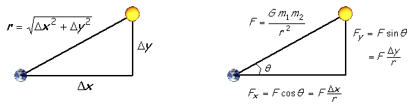
Homework 3 // Due at Lecture Monday, October 12 2010

Perform this assignment on the x86-64 Nehalem-based systems ale-01.cs.wisc.edu and ale-02.cs.wisc.edu.

You should do this assignment alone. No late assignments.

Purpose

The purpose of this assignment is to explore the features of Intel's (R) Thread Building Blocks multithreading package, including task management, synchronization, and concurrent data structures.

Programming Environment: OpenMP & TBB

OpenMP is a shared-memory programming model that attempts to automatically parallelize code that was written in a (mostly) serial fashion. OpenMP makes extensive use of compiler directives and optimizations, in addition to its own runtime library.

If you have not already done so, it is suggested that you review the OpenMP references provided in the Reading List.

OpenMP uses a Fork/Join model similar to that of P-Threads, but Fork/Join events are more frequent in OpenMP than in most P-Thread based programs. Most OpenMP programs consist of interleaved parallel and sequential sections, with "Fork" events occurring at the start of each parallel section, and "Join" events at the end of each parallel section. In non-parallel sections, only the "master thread" executes.

In order to use the OpenMP environment on ale, students should use the icc complier. Any source files that employ OpenMP directives or library calls must include the omp.h header file. Additionally, the flag -openmp must be passed to icc for both compilation and linking.

A set of OpenMP example programs are available for review here.

Intel's Thread Building Blocks (TBB) package provides a host of useful paralllel programmer services, including some of the same loop parallelization options provided by OpenMP and task-parallel tools like Cilk. Intel provides a handy Getting Started Guide that is available at the link above under the Documentation tab, which will show you everything you need to know about TBB for the purposes of this assignment. You will find the Tutorial document very useful as well.

Programming Task: N-Body Simulation

An n-body simulation calculates the gravitational effects of the masses of n bodies on each others' positions and velocities. The final values are generated by incrementally updating the bodies over many small time-steps. We will look at two approaches to this problem. First, we will calculate the pairwise force exerted on each particle by all other particles, an O(n²) operation. Second, we will use an quadtree data structure to implement an 0(n log n) approximation algorithm. A great overview of the O (n log n) algorithm can be found here. For simplicity, we will model the bodies in a two-dimensional space.

The physics. We review the equations governing the motion of the particles according to Newton's laws of motion and gravitation. Don't worry if your physics is a bit rusty; all of the necessary formulas are included below. We already know each particle's position (r_x, r_y) and velocity (v_x, v_y). To model the dynamics of the system, we must determine the net force exerted on each particle.

• Pairwise force. Newton's law of universal gravitation asserts that the strength of the gravitational force between two particles is given by the product of their masses divided by the square of the distance between them, scaled by the gravitational constant G, which is 6.67 × 10^-11 N m² / kg². The pull of one particle towards another acts on the line between them. Since we will be using Cartesian coordinates to represent the position of a particle, it is convenient to break up the force into its x and y components (F_x, F_y) as illustrated below.
  
• Net force. The principle of superposition says that the net force acting on a particle in the x or y direction is the sum of the pairwise forces acting on the particle in that direction.

• Acceleration. Newton's second law of motion postulates that the accelerations in the x and y directions are given by: a_x = F_x / m, a_y = F_y / m.

The numerics.  We use the leapfrog finite difference approximation scheme to numerically integrate the above equations: this is the basis for most astrophysical simulations of gravitational systems. In the leapfrog scheme, we discretize time, and update the time variable t in increments of the time quantum Δt. We maintain the position and velocity of each particle, but they are half a time step out of phase (which explains the name leapfrog). The steps below illustrate how to evolve the positions and velocities of the particles.

For each particle:

1. Calculate the net force acting on it at time t using Newton's law of gravitation and the principle of superposition.

2. Calculate its acceleration (a_x, a_y) at time t using its force at time t and Newton's second law of motion.

3. Calculate its velocity at time t + Δt / 2 by using its acceleration at time t and its velocity (v_x, v_y) at time t - Δt / 2. Assume that the acceleration remains constant in this interval, so that the updated velocity is:   v_x = v_x + Δt a_x,   v_y = v_y + Δt a_y.

4. Calculate its position at time t + Δt by using its velocity at time t + Δt / 2 and its position at time t. Assume that the velocity remains constant in the interval from t to t + Δt, so that the resulting position is given by r_x = r_x + Δt v_x,   r_y = r_y + Δt v_y. Note that because of the leapfrog scheme, the constant velocity we are using is the one estimated at the middle of the interval rather than either of the endpoints.

As you would expect, the simulation is more accurate when Δt is very small, but this comes at the price of more computation.

Problem 1: Parallelize O(n²) N-Body

For this problem, you are to parallelize the O(n²) pairwise version of the N-body simulation using both OpenMP and TBB. You may use any of the TBB mechanisms, though you may find parallel_for most useful.

You are required to make an argument that your n-body implementations are correct. A good way to do this is to initialize the bodies to a special-case starting condition, and then show that after a number of time steps the state of the grid exhibits symmetry or some other expected property. You need not prove your implementation's correctness in the literal sense. However, please annotate any simulation outputs clearly.

Problem 2: Parallelize O(n log n) N-Body

Everything in TBB is a task. In this problem, you are to explore the many ways to utilize tasks by parallelizing the O(n log n) version of the N-body simulation. You will find that this version of the simulation heavily utilizes recursion; recursive calls often make great tasks.

In this problem you should experiment with the granularity of tasks. Too many tasks leads to high overheads and too few tasks parallelize poorly. You should incrementally modify your parallization strategy until you find one that is a good balance between overhead and parallelization that leads to good performance.

Problem 3: Analysis of N-Body Algorithms

In this section, you will analyze the performance of your three N-Body implementations.

Part A: Plot the normalized (versus the serial n² version) speedups of programs 1a and 1b on the same graph for N=[1,2,4,8,16] threads and for 512 bodies and 5000 timesteps. The value of dt is irrelevant to studying scalability: with the number of time steps held constant, it only affects the length of time simulated, not the duration of the simulation itself. Thus you may choose any value you like.

Part B: Plot the normalized (versus the respective serial version of n-body) speedups of Programs 1a, 1b, and 2 on N=[1,2,4,8,16] threads for 512 bodies and 5000 time steps.

Part C: Plot the execution time of Programs 1a, 1b, and 2 on N=[1,2,4,8,16] threads for 512 bodies and 5000 time steps on the same graph.

Problem 4: Questions (Submission Credit)

1. Comment on the TBB programming environment. Specifically compare and contrast it to pthreads. Which do you like better, and why?
2. Did you like OpenMP or TBB better? In problem 1, which had better performance? Why do you think that is?
3. Desribe your parallelization strategy for both problems 1 and 2. Which was easier? Which scaled better?
4. Comment on the relative speedups between parallelization strategies. Was the speedup worth the additional effort of the more difficult program?

Source Code

We will provide you with working implementations of both n² and n log n n-body simulations. They are stored in a mercurial repository. You can check it out with the following command:

hg clone /p/course/cs758-david/public/repo/hw3

This assigment can be completed by implementing new subclasses of the NbodySimulator class. See the existing code/Makefile for more direction.

It is your responsibility to get TBB installed and working in your working directory. All students should use TBB version 3.0, available on the TBB website.

Tips and Tricks

• Start early.
• Make use of the demo programs provided.
• Read TBB's Tutorial
• Don't forget to add -ltbb and other useful switches in the provided Makefile
• Don't forget to source TBB's environment variables!

What to Hand In

Please turn this homework in on paper at the beginning of lecture. You must include:

• A printout of your parallel implementation of Programs 1a and 1b. Only include relevant code.
• A printout of the parallel implementation of Program 2. Only include relevant code.
• Arguments for the correctness of Programs 1 and 2.
• The plots as described in Problem 3a and 3b, including labels describing your data.
• Answers to the questions in Problem 4.

Important: Include your name on EVERY page.