Why Reason Probabilistically?

• In many problem domains it isn't possible to create complete, consistent models of the world. Therefore agents (and people) must act in uncertain worlds (which the real world is).
• Want an agent to make rational decisions even when there is not enough information to prove that an action will work.
• Some of the reasons for reasoning under uncertainty:
  • True uncertainty. E.g., flipping a coin.
  • Theoretical ignorance. There is no complete theory which is known about the problem domain. E.g., medical diagnosis.
  • Laziness. The space of relevant factors is very large, and would require too much work to list the complete set of antecedents and consequents. Furthermore, it would be too hard to use the enormous rules that resulted.
  • Practical ignorance. Uncertain about a particular individual in the domain because all of the information necessary for that individual has not been collected.
• Probability theory will serve as the formal language for representing and reasoning with uncertain knowledge.

Representing Belief about Propositions

• Rather than reasoning about the truth or falsity of a proposition, reason about the belief that a proposition or event is true or false
• For each primitive proposition or event, attach a degree of belief to the sentence
• Use probability theory as a formal means of manipulating degrees of belief
• Given a proposition, A, assign a probability, P(A), such that 0 <= P(A) <= 1, where if A is true, P(A)=1, and if A is false, P(A)=0. Proposition A must be either true or false, but P(A) summarizes our degree of belief in A being true/false.
• Examples
  • P(Weather=Sunny) = 0.7 means that we believe that the weather will be Sunny with 70% certainty. In this case Weather is a random variable that can take on values in a domain such as {Sunny, Rainy, Snowy, Cloudy}.
  • P(Cavity=True) = 0.05 means that we believe there is a 5% chance that a person has a cavity. Cavity is a Boolean random variable since it can take on possible values True and False.
  • Example: P(A=a ^ B=b) = P(A=a, B=b) = 0.2, where A=My_Mood, a=happy, B=Weather, and b=rainy, means that there is a 20% chance that when it's raining my mood is happy.
• Obtaining and Interpreting Probabilities
  There are several senses in which probabilities can be obtained and interpreted, among them the following:
  • Frequentist Interpretation
    The probability is a property of a population of similar events. E.g., if set S = P union N, and P intersection N is the empty set, then the probability of an object being in set P is |P|/|S|. Hence, in this interpretation probabilities come from experiments and determining the population associated with a given proposition.
  • Subjectivist Interpretation
    A subjective degree of belief in a proposition or the occurrence of an event. E.g., the probability that you'll pass the Final Exam based on your own subjective evaluation of the amount of studying you've done and your understanding of the material. Hence, in this interpretation probabilities characterize the agent's beliefs.

• We will assume that in a given problem domain, the programmer and expert identify all of the relevant propositional variables that are needed to reason about the domain. Each of these will be represented as a random variable, i.e., a variable that can take on values from a set of mutually exclusive and exhaustive values called the sample space or partition of the random variable. Usually this will mean a sample space {True, False}. For example, the proposition Cavity has possible values True and False indicating whether a given patient has a cavity or not. A random variable that has True and False as its possible values is called a Boolean random variable.

  More generally, propositions can include the equality predicate with random variables and the possible values they can have. For example, we might have a random variable Color with possible values red, green, blue, and other. Then P(Color=red) indicates the likelihood that the color of a given object is red. Similarly, for Boolean random variables we can ask P(A=True), which is abbreviated to P(A), and P(A=False), which is abbreviated to P(~A).

Axioms of Probability Theory

• 0 <= P(A=a) <= 1 for all a in sample space of A
• P(True)=1, P(False)=0
• P(A v B) = P(A) + P(B) - P(A ^ B)

• P(~A) = 1 - P(A)
• P(A) = P(A ^ B) + P(A ^ ~B)
• Sum{P(A=a)} = 1, where the sum is over all possible values a in the sample space of A

Joint Probability Distribution

For example, consider a domain described by three Boolean random variables, Bird, Flier, and Young. Then we can enumerate a table showing all possible interpretations and associated probabilities:

Bird	Flier	Young	Probability
T	T	T	0.0
T	T	F	0.2
T	F	T	0.04
T	F	F	0.01
F	T	T	0.01
F	T	F	0.01
F	F	T	0.23
F	F	F	0.5

Notice that there are 8 rows in the above table representing the fact that there are 2³ ways to assign values to the three Boolean variables. More generally, with n Boolean variables the table will be of size 2ⁿ. And if n variables each had k possible values, then the table would be size kⁿ.

Also notice that the sum of the probabilities in the right column must equal 1 since we know that the set of all possible values for each variable are known. This means that for n Boolean random variables, the table has 2ⁿ-1 values that must be determined to completely fill in the table.

If all of the probabilities are known for a full joint probability distribution table, then we can compute any probabilistic statement about the domain. For example, using the table above, we can compute

• P(Bird=T) = P(B) = 0.0 + 0.2 + 0.04 + 0.01 = 0.25
• P(Bird=T, Flier=F) = P(B, ~F) = P(B, ~F, Y) + F(B, ~F, ~Y) = 0.04 + 0.01 = 0.05

Conditional Probabilities

• Conditional probabilities are key for reasoning because they formalize the process of accumulating evidence and updating probabilities based on new evidence. For example, if we know there is a 4% chance of a person having a cavity, we can represent this as the prior (aka unconditional) probability P(Cavity)=0.04. Say that person now has a symptom of a toothache, we'd like to know what is the posterior probability of a Cavity given this new evidence. That is, compute P(Cavity | Toothache).

• If P(A|B) = 1, this is equivalent to the sentence in Propositional Logic B => A. Similarly, if P(A|B) =0.9, then this is like saying B => A with 90% certainty. In other words, we've made implication fuzzy because it's not absolutely certain.

• Given several measurements and other "evidence", E1, ..., Ek, we will formulate queries as P(Q | E1, E2, ..., Ek) meaning "what is the degree of belief that Q is true given that we know E1, ..., Ek and nothing else."

• Conditional probability is defined as: P(A|B) = P(A ^ B)/P(B) = P(A,B)/P(B)
  One way of looking at this definition is as a normalized (using P(B)) joint probability (P(A,B)).

• Example Computing Conditional Probability from the Joint Probability Distribution
  Say we want to compute P(~Bird | Flier) and we know the full joint probability distribution function given above. We can do this as follows:

     P(~B|F) = P(~B,F) / P(F)
  	   = (P(~B,F,Y) + P(~B,F,~Y)) / P(F)
             = (.01 + .01)/P(F)
  

  Next, we could either compute the marginal probability P(F) from the full joint probability distribution, or, as is more commonly done, we could do it by using a process called normalization, which first requires computing

     P(B|F) = P(B,F) / P(F)
  	  = (P(B,F,Y) + P(B,F,~Y)) / P(F)
  	  = (0.0 + 0.2)/P(F)
  

  Now we also know that P(~B|F) + P(B|F) = 1, so substituting from above and solving for P(F) we get P(F) = 0.22. Hence, P(~B|F) = 0.02/0.22 = 0.091.

  While this is an effective procedure for computing conditional probabilities, it is intractable in general because it means that we must compute and store the full joint probability distribution table, which is exponential in size.

• Some important rules related to conditional probability are:
  • Rewriting the definition of conditional probability, we get the Product Rule: P(A,B) = P(A|B)P(B)
  • Chain Rule: P(A,B,C,D) = P(A|B,C,D)P(B|C,D)P(C|D)P(D), which generalizes the product rule for a joint probability of an arbitrary number of variables. Note that ordering the variables results in a different expression, but all have the same resulting value.
  • Conditionalized version of the Chain Rule: P(A,B|C) = P(A|B,C)P(B|C)
  • Bayes's Rule: P(A|B) = (P(A)P(B|A))/P(B), which can be written as follows to more clearly emphasize the "updating" aspect of the rule: P(A|B) = P(A) * [P(B|A)/P(B)] Note: The terms P(A) and P(B) are called the prior (or marginal) probabilities. The term P(A|B) is called the posterior probability because it is derived from or depends on the value of B.
  • Conditionalized version of Bayes's Rule: P(A|B,C) = P(B|A,C)P(A|C)/P(B|C)
  • Conditioning (aka Addition) Rule: P(A) = Sum{P(A|B=b)P(B=b)} where the sum is over all possible values b in the sample space of B.
  • P(~B|A) = 1 - P(B|A)

Combining Multiple Evidence using the Joint Probability Distribution

P(~Bird | Flier, ~Young) = P(~B,F,~Y) / (P(~B,F,~Y) + P(B,F,~Y))
                         = .01 / (.01 + .2)
			 = .048

In general, P(V1=v1, ..., Vk=vk | Vk+1=vk+1, ..., Vn=vn) = sum of all entries where V1=v1, ..., Vn=vn divided by the sum of all entries where Vk+1=vk+1, ..., Vn=vn.

While this method will work for any conditional probability involving arbitrary known evidence, it is again intractable because it requires an exponentially large table in the form of the full joint probability distribution.

Using Bayes's Rule

• Bayes's Rule is the basis for probabilistic reasoning because given a prior model of the world in the form of P(A) and a new piece of evidence B, Bayes's Rule says how the new piece of evidence decreases my ignorance about the world by defining P(A|B).

• Why use Bayes's Rule?
  Often want to know P(A|B) but only have access to P(B|A). For example, let S represent the proposition that a given patient has a stiff neck, and let M represent the proposition that the patient has meningitis. The doctor and patient may like to know P(M|S), but obtaining this information from the general population is difficult. Besides it could change significantly over time given epidemics or other seasonal factors. On the other hand, doctors may be able to accumulate statistics that define P(S|M). So, for example, if P(M) = 1/50,000, P(S) = 1/20, and P(S|M) = 1/2, then using Bayes's Rule says that P(M|S) = 1/5000 = .0002

• Combining Multiple Evidence using Bayes's Rule
  Generalizing Bayes's Rule for two pieces of evidence, B and C, we get:

  P(A|B,C) = ((P(A)P(B,C | A))/P(B,C)
             = P(A) * [P(B|A)/P(B)] * [P(C | A,B)/P(C|B)]
  

  Again, this shows how the conditional probability of A is updated given B and C. The problem is that it may be hard in general to obtain or compute P(C | A,B). But this difficulty is circumvented if we know evidence B and C are conditionally independent or unconditionally independent.
  • A is (unconditionally) independent of B if P(A|B) = P(A). In this case, P(A,B) = P(A)P(B).
  • A is conditionally independent of B given C if P(A|B,C) = P(A|C) and, symmetrically, P(B|A,C) = P(B|C). What this means is that if we know P(A|C), we also know P(A|B,C), so we don't need to store this case. Furthermore, it also means that P(A,B|C) = P(A|C)P(B|C).

• Bayes's Rule with Multiple, Independent Evidence
  Assuming conditional independence of B and C given A, we can simplify Bayes's Rule for two pieces of evidence B and C:

  P(A | B,C) = (P(A)P(B,C | A))/P(B,C)
             = (P(A)P(B|A)P(C|A))/(P(B)P(C|B))
             = P(A) * [P(B|A)/P(B)] * [P(C|A)/P(C|B)]
             = (P(A) * P(B|A) * P(C|A))/P(B,C)
  

  The above expression that assumes conditional indepedence is used to define a Naive Bayes Classifier in the following way. Say we have a random variable, C, which represents the possible ways to classify an input pattern of features that have been measured. The domain of C is the set of possible classifications, e.g., it might be the possible diagnoses in a medical domain. Say the possible values for C are {a,b,c}, and the features we have measured are E1=e1, E2=e2, ..., En=en. Then we can compute P(C=a | E1=e1, ..., En=en), P(C=b | E1=e1, ..., En=en) and P(C=c | E1=e1, ..., En=en) assuming E1, ..., En are conditionally independent given C. Since for each value of C the denominators are the same above, they can be ignored. So, for example P(C=a | E1=e1, ..., En=en) = P(C=a) * P(E1=e1 | C=a) * P(E2=e2 | C=a) * ... * P(En=en | C=a) Choose the value for C that gives the maximum probability. Finally, since only relative values are needed and probabilities are often very small, it is common to compute the sum of logarithms of the probabilities: log P(C=a | E1=e1, ..., En=en) = log P(C=a) + log P(E1=e1 | C=a) + ... + log P(En=en | C=a).

  If B and C are (unconditionally) independent, then P(C|B) = P(C), so

  P(A | B,C) = P(A) * [P(B|A)/P(B)] * [P(C|A)/P(C)]
  

• Example
  Consider the medical domain consisting of three Boolean variables: PickledLiver, Jaundice, Bloodshot, where the first indicates if a given patient has the "disease" PickledLiver, and the second and third describe symptoms of the patient. We'll assume that Jaundice and Bloodshot are independent.

  The doctor wants to determine the likelihood that the patient has a PickledLiver. Based on no other information, she knows that the prior probability P(PickledLiver) = 10^-17. So, this represents the doctor's initial belief in this diagnosis. However, after examination, she determines that the patient has jaundice. She knows that P(Jaundice) = 2^-10 and P(Jaundice | PickledLiver) = 2^-3, so she computes the new updated probability in the patient having PickledLiver as:

  P(PickledLiver | Jaundice) = P(P)P(J|P)/P(J)
                             = (2-17 * 2-3)/2-10
                             = 2-10
  

  So, based on this new evidence, the doctor increases her belief in this diagnosis from 2^-17 to 2^-10. Next, she determines that the patient's eyes are bloodshot, so now we need to add this new piece of evidence and update the probability of PickledLiver given Jaundice and Bloodshot. Say, P(Bloodshot) = 2^-6 and P(Bloodshot | PickledLiver) = 2^-1. Then, she computes the new conditional probability:

  P(PickledLiver | Jaundice, Bloodshot) = (P(P)P(J|P)P(B|P))/(P(J)P(B))
                                        = 2-10 * [2-1 / 2-6]
                                        = 2-5
  

  So, after taking both symptoms into account, the doctor's belief that the patient has a PickledLiver is 2^-5.

Bayesian Networks (aka Belief Networks)

• Bayesian Networks, also known as Bayes Nets, Belief Nets, Causal Nets, and Probability Nets, are a space-efficient data structure for encoding all of the information in the full joint probability distribution for the set of random variables defining a domain. That is, from the Bayesian Net one can compute any value in the full joint probability distribution of the set of random variables.
• Represents all of the direct causal relationships between variables
• Intuitively, to construct a Bayesian net for a given set of variables, draw arcs from cause variables to immediate effects.
• Space efficient because it exploits the fact that in many real-world problem domains the dependencies between variables are generally local, so there are a lot of conditionally independent variables
• Captures both qualitative and quantitative relationships between variables
• Can be used to reason
  • Forward (top-down) from causes to effects -- predictive reasoning (aka causal reasoning)
  • Backward (bottom-up) from effects to causes -- diagnostic reasoning

• Formally, a Bayesian Net is a directed, acyclic graph (DAG), where there is a node for each random variable, and a directed arc from A to B whenever A is a direct causal influence on B. Thus the arcs represent direct causal relationships and the nodes represent states of affairs. The occurrence of A provides support for B, and vice versa. The backward influence is call "diagnostic" or "evidential" support for A due to the occurrence of B.
• Each node A in a net is conditionally independent of any subset of nodes that are not descendants of A given the parents of A.

Net Topology Reflects Conditional Independence Assumptions

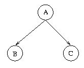
• Conditional independence defines local net structure. For example, if B and C are conditionally independent given A, then by definition P(C|A,B) = P(C|A) and, symmetrically, P(B|A,C) = P(B|A). Intuitively, think of A as the direct cause of both B and C. In a Bayesian Net this will be represented by the local structure:
  

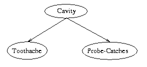
  For example, in the dentist example in the textbook, having a Cavity causes both a Toothache and the dental probe to Catch, but these two events are conditionally independent given Cavity. That is, if we know nothing about whether or not someone has a Cavity, then Toothache and Catch are dependent. But as soon as we definitely know the person has a cavity or not, then knowing that the person has a Toothache as well has no effect on whether Catch is true. This conditional independence relationship will be reflected in the Bayesian Net topology as:

  

• In general, we will construct the net so that given its parents, a node is conditionally independent of the rest of the net variables. That is,

  P(X1=x1, ..., Xn=xn) = P(xi | Parents(Xi)) * ... * P(xn | Parents(Xn))

  Hence, we don't need the full joint probability distribution, only conditionals relative to the parent variables.

• Example (From (Charniak, 1991))

  Consider the problem domain in which when I go home I want to know if someone in my family is home before I go in. Let's say I know the following information: (1) Why my wife leaves the house, she often (but not always) turns on the outside light. (She also sometimes turns the light on when she's expecting a guest.) (2) When nobody is home, the dog is often left outside. (3) If the dog has bowel-troubles, it is also often left outside. (4) If the dog is outside, I will probably hear it barking (though it might not bark, or I might hear a different dog barking and think it's my dog). Given this information, define the following five Boolean random variables:

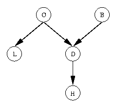
  O: Everyone is Out of the house
  L: The Light is on
  D: The Dog is outside
  B: The dog has Bowel troubles
  H: I can Hear the dog barking
  

  From this information, the following direct causal influences seem appropriate:

  1. H is only directly influenced by D. Hence H is conditionally independent of L, O and B given D.
  2. D is only directly influenced by O and B. Hence D is conditionally independent of L given O and B.
  3. L is only directly influenced by O. Hence L is conditionally independent of D, H and B given O.
  4. O and B are independent.

  Based on the above, the following is a Bayesian Net that represents these direct causal relationships (though it is important to note that these causal connections are not absolute, i.e., they are not implications):

  

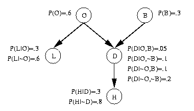
  Next, the following quantitative information is added to the net; this information is usually given by an expert or determined empirically from training data.

  • For each root node (i.e., node without any parents), the prior probability of the random variable associated with the node is determined and stored there
  • For each non-root node, the conditional probabilities of the node's variable given all possible combinations of its immediate parent nodes are determined. This results in a conditional probability table (CPT) at each non-root node.

  Doing this for the above example, we get the following Bayesian Net:

  

  Notice that in this example, a total of 10 probabilities are computed and stored in the net, whereas the full joint probability distribution would require a table containing 2⁵ = 32 probabilities. The reduction is due to the conditional independence of many variables.

  Two variables that are not directly connected by an arc can still affect each other. For example, B and H are not (unconditionally) independent, but H does not directly depend on B.

  Given a Bayesian Net, we can easily read off the conditional independence relations that are represented. Specifically, each node, V, is conditionally independent of all nodes that are not descendants of V, given V's parents. For example, in the above example H is conditionally independent of B, O, and L given D. So, P(H | B,D,O,L) = P(H | D).

Building a Bayesian Net

More formally, the following algorithm constructs a Bayesian Net:

1. Identify a set of random variables that describe the given problem domain
2. Choose an ordering for them: X1, ..., Xn
3. for i=1 to n do
   1. Add a new node for Xi to the net
   2. Set Parents(Xi) to be the minimal set of already added nodes such that we have conditional independence of Xi and all other members of {X1, ..., Xi-1} given Parents(Xi)
   3. Add a directed arc from each node in Parents(Xi) to Xi
   4. If Xi has at least one parent, then define a conditional probability table at Xi: P(Xi=x | possible assignments to Parents(Xi)). Otherwise, define a prior probability at Xi: P(Xi)

Notes about this algorithm:

• There is not, in general, a unique Bayesian Net for a given set of random variables. But all represent the same information in that from any net constructed every entry in the joint probability distribution can be computed.
• The "best" net is constructed if in Step 2 the variables are topologically sorted first. That is, each variable comes before all of its children. So, the first nodes should be the roots, then the nodes they directly influence, and so on.
• The algorithm will not construct a net that is illegal in the sense of violating the rules of probability.

Computing Joint Probabilities from a Bayesian Net

Goal: Compute P(B,~O,D,~L,H)

P(B,~O,D,~L,H) = P(H,~L,D,~O,B)
     = P(H | ~L,D,~O,B) * P(~L,D,~O,B)            by Product Rule
     = P(H|D) * P(~L,D,~O,B)                      by Conditional Independence of H and
                                                       L,O, and B given D
     = P(H|D) P(~L | D,~O,B) P(D,~O,B)            by Product Rule
     = P(H|D) P(~L|~O) P(D,~O,B)                  by Conditional Independence of L and D,
                                                       and L and B, given O
     = P(H|D) P(~L|~O) P(D | ~O,B) P(~O,B)        by Product Rule
     = P(H|D) P(~L|~O) P(D|~O,B) P(~O | B) P(B)   by Product Rule
     = P(H|D) P(~L|~O) P(D|~O,B) P(~O) P(B)       by Independence of O and B
     = (.3)(1 - .6)(.1)(1 - .6)(.3)
     = 0.00144

where all of the numeric values are available directly in the Bayesian Net (since P(~A|B) = 1 - P(A|B)).

Computing Conditional Probabilities from a Bayesian Net

Causal (Top-Down) Inference

Consider our "home domain" and the problem of computing P(D|B), i.e., what is the probability that my dog is outside when it has bowel troubles? We can solve this problem as follows:

1. Apply the Product Rule and Marginalization

   P(D|B) = P(D,B)/P(B)                   by the Product Rule
          = (P(D,B,O) + P(D,B,~O))/P(B)   by marginalizing P(D,B)
          = P(D,B,O)/P(B) + P(D,B,~O)/P(B)
          = P(D,O|B) + P(D,~O|B)
   

2. Apply the conditionalized version of the chain rule, i.e., P(A,B|C) = P(A|B,C)P(B|C), to obtain

   P(D|B) = P(D|O,B)P(O|B) + P(D|~O,B)P(~O|B)
   

3. Since O and B are independent by the network, we know P(O|B)=P(O) and P(~O|B)=P(~O). This means we now have

   P(D|B) = P(D|O,B)P(O) + P(D|~O,B)P(~O)
          = (.05)(.6) + (.1)(1 - .6)
          = 0.07
   

In general, for this case we first rewrite the goal conditional probability of query variable Q in terms of Q and all of its parents (that are not evidence) given the evidence. Second, re-express each joint probability back to the probability of Q given all of its parents. Third, look up in the Bayesian Net the required values.

Diagnostic (Bottom-Up) Inference

For example, consider the "home domain" again and the problem of computing P(~B|~D). That is, if the dog is not outside, what is the probability that the dog has bowel troubles?

1. First, use Bayes's Rule:

   P(~B|~D) = P(~D|~B)P(~B)/P(~D)
   

2. We can look up in the Bayesian Net the value of P(~B) = 1 - .3 = .7. Next, compute P(~D|~B) using the causal inference method described above. Here we get

   P(~L|~B) = P(~D,O|~B) + P(~D,~O|~B)
            = P(~D|O,~B)P(O|~B) + P(~D|~O,~B)P(~O|~B)
            = P(~D|O,~B)P(O) + P(~D|~O,~B)P(~O)
            = (.9)(.6) + (.8)(.4)
            = 0.86
   

   So, P(~B|~D) = (.86)(.7)/P(~D) = .602/P(~D).

3. To avoid computing the prior probability, P(~D), of symptom D, we can use normalization, which requires computing P(B|~D). That is, P(B|~D) = P(~D|B)P(B)/P(~D) by Bayes's Rule, and P(B)=.3 from the Bayesian Net. Now compute P(~D|B) as follows:

   P(~D|B) = P(~D,O|B) + P(~D,~O|B)
           = P(~D|O,B)P(O|B) + P(~D|~O,B)P(~O|B)
           = P(~D|O,B)P(O) + P(~D|~O,B)P(~O)
           = (.95)(.6) + (.9)(.4)
           = 0.93
   

   So, P(B|~D) = (.93)(.3)/P(~D) = .279/P(~D). Since P(~B|~D) + P(B|~D) = 1, we have .602/P(~D) + .279/P(~D) = 1, and so P(~D) = .881. Thus, P(~B|~D) = .602/.881 = .683.

In general, diagnostic inference problems are solved by converting them to causal inference problems using Bayes's Rule, and then proceeding as before.

Summary

• We have a methodology for building a Bayesian Net
• The Bayesian Net is compact in that it doesn't usually require exponential storage to hold all of the information in the joint probability distribution table
• We can compute the probability of any given assignment of truth values to the variables (i.e., compute the probability for an entry in the joint probability distribution table). And this computation is fast -- linear in the number of nodes in the net.
• But, many queries of interest are conditional, of the form:
  P(Q | E1, E2, ..., Ek)
  That is, given a set of values for selected random variables, E1, ..., Ek, representing a set of evidence gathered, compute the posterior probability of the query variable Q. In general, this requires enumerating all of the "matching" cases in the joint, which takes time exponential in the number of variables. So, general querying using a Bayesian Net is NP-hard. But, certain special cases (tree-structured nets called polytrees, where there is just one path, along arcs in either direction, between any two nodes in the Net) take polynomial time.
• For an alternative introductory description of Bayesian Nets, see the article "Bayesian Networks Without Tears" by E. Charniak, AI Magazine 12(4): Winter 1991, 50-63.

Copyright © 1996-2003 by Charles R. Dyer. All rights reserved.