notes
type “?” to learn navigation, HOME
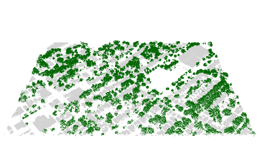
Finding the trees for the urban forest
I recently found the lidR package, an incredible tool for working
with lidar data in R. I used it to separate trees from buildings.
See my github repository for the code and explanation. Below is an
example of the results.
Stan on CHTC.
The final assignment for the open science grid user school was to write about how we could take what we learned at the school and apply it to our work. I decided to figure out how to get Stan, “a state-of-the-art platform for statistical modeling and high-performance statistical computation”, running on a high throughput system. I hope the github repo I created will be helpful for my research and others trying to run Stan on a cluster.
https://github.com/TedwardErker/chtc_stan
My second paper published!
I’m very proud of this one. It’s years of work cut out and the rest condensed into a small space. In addition to my advisor, Phil Townsend, I’m grateful to Chris Kucharik for his guidance.
The review process really helped improve the text to be more clear. I submitted a version of this paper for Steve Carpenter’s Ecosystem Concepts class. He didn’t think very much of the paper and said that it would be unlikely to be published because the statistical significance was so low. At first I was bothered by this comment because actually the results were very clear statistically - it was the effect size that was small. I thought Steve was missing the point. But, rereading the paper I realized the burden was mine to guide the reader to understand the nature of the study, the data, and the relevance to science and society. The final product is not perfect, but it’s a big improvement due in part to Steve’s frank criticism.
p.s. there is a small typo in the text introduced by the editor that I didn’t catch during the final proofs. So it goes.
Open Science Grid User School

This July I participated in the Open Science Grid User School. It was an incredible learning opportunity. With loads of hands-on exercises over the course of a week we learned how to harness the power of a high throughput system. I had been familiar with using HTCondor from my previous work, but this solidified things and allowed me to move to next level of implementation. It was a great group of learners and teachers.
My first paper published!
Finally. This took too long, but here you go world.
My first review life
I got this sweet email:
Dear Mr. Erker,
Thank you for your review of this manuscript. Your review is an important part of the publication process. Serving as a reviewer is a time consuming and often thankless job. Please be assured that your help is appreciated.
Plus this corny certificate:
Stat Consultant Job life
I’m excited to say that in March I will start part time as a statistical consultant in the CALS stat consulting lab. Find the form to sign up for a consultation here :) .
AGU Fall meeting 2018 Poster UrbanTrees

Unfortunately, I wasn’t able to attend the conference, so Phil presented my poster for me. I was standing by to video chat with anyone interested, but there were no takers :(. A few reporters were interested - one even called me later to ask some questions. But I don’t think any story will come of it. Still, it was very neat to share my work with a large audience. Find a larger image here: Urban shade trees may be an atmospheric carbon source for much of the US. This work is now in review at Environmental Research Letters.
Tree shadows on a house visualization

I made these to illustrate the patterns of shade that trees provide to houses throughout the year at the latitude of Madison, WI.
I am a master of science now. life statistics
Today I defended my biometry MS project (presentation here). It felt good to be recognized for all the learning I’ve done in the past many years. I am now officially a master of science. Now back to work on my PhD.
SESYNC Workshop in Annapolis travel UrbanTrees
This week I participated in a National Socio-Environmental Synthesis Center (SESYNC) pursuit workshop. Drs. Lea Johnson and Michelle Johnson brought together a team of around a dozen or so social scientists, natural scientists and managers to plan a study of urban forest patches in Chicago and the Megalopolis of the east coast (Washington D.C., Baltimore, Philidelphia, and NYC). It was an amazing experience to meet people from all over who are as interested in urban trees as I am. We had loads of constructive discussion and I’m excited for the follow-up workshops in 2019.
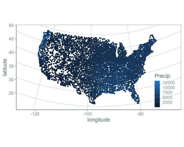
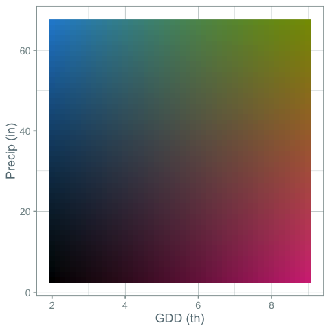
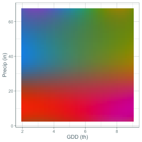
A 2-dimensional color palette visualization
Color scales are usually applied to one variable in a plot. For example:
or
 (Code for these and the below figures is in this repository).
But what if you wanted to show changes in both precipitation and growing degree days at the same time with color. This would require a kind of 2-d color palette. Something like this:
Here’s a map using this color scheme:
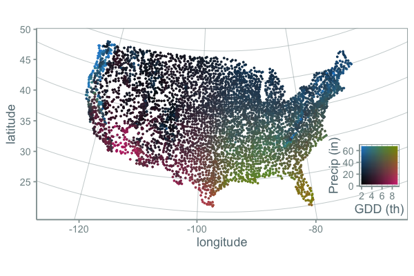
This is nice, but color interpolation is hard to do. There is a fair bit of grey around mean GDD and mean precipitation. I think this works, but could be more informative. Here’s another palette:
and the map:
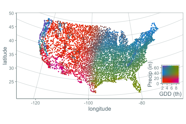
While this palette is more of a mess of colors and the gradients may break some rules about how palettes should be made to maximize a person’s ability to accurately compare of values, I find it more informative. It is clear that the variation of gdd and precip across the US is a continuous gradient, but clear climate lines break out in places you might expect.
One problem with this approach is that there are actually many weather stations with precip greater than 60 inches per year and other stations that fall outside of the scale. What ggplot does by default in these cases is it turns these points grey, which is what I probably should have done. But instead I assigned these points the closest color because I was more interested in general patterns (high, medium, low) rather than the specific number.
One way around this problem is shown in the figure below:
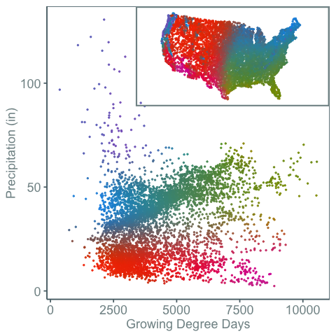
Here the weather stations are plotted in climate space and geographic space. Color then connects the two. This shows that the purple colored weather stations can have very high precipitation levels. It also shows how weather spaces are distributed in both climate and geographic space.
Google Scholar Results In a Nice Table computing
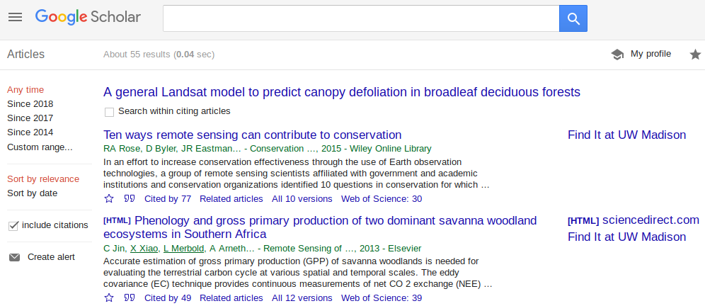
Say you want to take a look at all the papers that cite a paper. You do a search, then click the “cited by” link. Now you can see all the papers that cited this one. Pretty neat. How can you get the results into a table that you can add notes to?
load libraries
  library(rvest)  # rvest for web scraping
  library(dplyr)  # dplyr for pipes (%>%)


  library(ascii)  # ascii for printing the dataframe in org mode
  options(asciiType = "org")
  org.ascii <- function(x) {
    suppressWarnings(print(ascii(x)))
  }
get urls of pages you want to download
The results aren’t all on a single page. So you need to give a vector of page urls.
Copy and paste the first and second page. By changing the number after “start=” in the second url, you can get the remaining pages.
    first.page <- c("https://scholar.google.com/scholar?cites=16900404805115852262&as_sdt=5,50&sciodt=0,50&hl=en")
    later.pages <- paste0("https://scholar.google.com/scholar?start=",seq(10,20,10),"&hl=en&as_sdt=5,50&sciodt=0,50&cites=16900404805115852262&scipsc=")
    pages <- c(first.page, later.pages)
extract the title; authors, publication, and year; and link using CSS classes
    out <- lapply(pages, function(page) {
      res <- read_html(page)
      title <- res %>%
          html_nodes(".gs_rt > a") %>%
          html_text()

      authors <- res %>%
          html_nodes(".gs_a") %>%
          html_text()

      link <- res %>%
        html_nodes(".gs_rt > a") %>%
        html_attr(name = "href")

     Sys.sleep(3) # wait 3 seconds

      o <- data_frame(title,authors,link)

    })

    df <- do.call("rbind", out)

    df <- mutate(df, link = paste0("[[",link,"][link]]"))  # make org mode link
print as org table
org.ascii(head(df))
| title | authors | link | |
|---|---|---|---|
| 1 | Ten ways remote sensing can contribute to conservation | RA Rose, D Byler, JR Eastman… - Conservation …, 2015 - Wiley Online Library | link |
| 2 | Phenology and gross primary production of two dominant savanna woodland ecosystems in Southern Africa | C Jin, X Xiao, L Merbold, A Arneth… - Remote Sensing of …, 2013 - Elsevier | link |
| 3 | The role of remote sensing in process-scaling studies of managed forest ecosystems | JG Masek, DJ Hayes, MJ Hughes, SP Healey… - Forest Ecology and …, 2015 - Elsevier | link |
| 4 | Remote monitoring of forest insect defoliation. A review | CDR Silva, AE Olthoff, JAD de la Mata… - Forest Systems, 2013 - dialnet.unirioja.es | link |
| 5 | Monitoring forest decline through remote sensing time series analysis | J Lambert, C Drenou, JP Denux, G Balent… - GIScience & remote …, 2013 - Taylor & Francis | link |
| 6 | Landsat remote sensing of forest windfall disturbance | M Baumann, M Ozdogan, PT Wolter, A Krylov… - Remote sensing of …, 2014 - Elsevier | link |
concluding thoughts
You might get this error:
Error in open.connection(x, “rb”) : HTTP error 503.
Google prevents massive automatic downloads for good reason. This code is meant to prevent the manual typing of page results into a table, not meant to scrape hundreds of results.
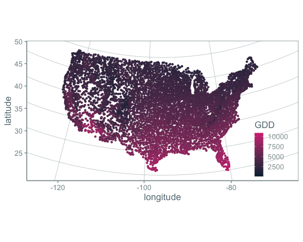
The U.S. Population in Heating and Cooling Degree Day Space
Madison, where I live now, is a cold city, especially when compared to my hometown St. Louis. Lake ice in Madison is measured in feet. Ice of any thickness on the man-made ponds of St. Louis is an ephemeral phenonmenon and ice of a few inches thick, a bygone memory from childhood. The summers of Madison are also cool. I used to complain after I left St. Louis that midnight summer bike rides in Madison lack something critical: the stored day’s heat radiating off the asphalt and into your skin as you ride through a blanket of humidity. But, as I write this, I’m sweating on my front porch. It doesn’t feel like I live in a cold city today.
For something related to my work, I was curious how Madison compared not just to St. Louis, but also to the rest of the country. What percent of Americans live in a climate that is as cold or colder than Madison? Where is the boundary between a “hot” and a “cold” city? And what percent of Americans live in cold places? hot places?
One way to measure this is with heating and cooling degree days. These are basically a measure of how much a place deviates from a balmy temperature, say 65 degrees farenheit. Cold places have more heating degree days (days when you need to turn on the heat) and hot places have more cooling degree days (days when you need to turn on the A/C).
I pulled climate data from NOAA and plotted it below. See this github repo for code.
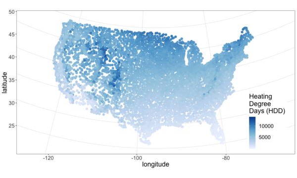
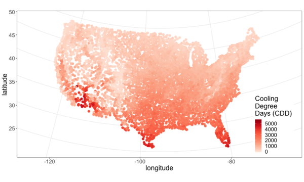
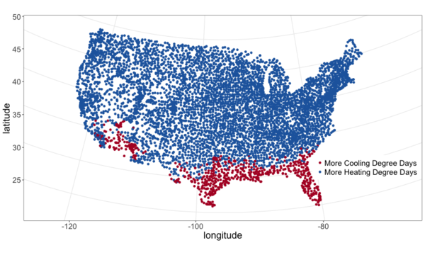
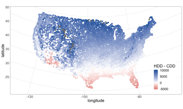
From the above maps it’s pretty clear that most of the continental U.S. is heating dominated (cold). This isn’t surprising, but it is neat to visualize and moves us closer to an approximation of what percent of Americans live in a heating or cooling dominated area. To answer that we need population data.
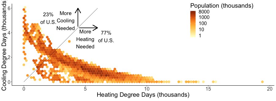
I joined census tract data with HDD and CDD based off the closest weather station to the tract’s centroid (more code here). Figure 22 plots the population in HDD and CDD space, using hexagon bins to prevent overplotting. The 1:1 line separates places that have more CDD than HDD from those that have more HDD than CDD.
A few key takeaways:
- slightly more than 3 out of every 4 Americans (77%) live in a heating dominated climate.
- Madison is a lot colder than most of the U.S.
- California, especially southern, is an exception to the strong inverse relationship between HDD and CDD across most of the country. They are not really hot and not really cold.
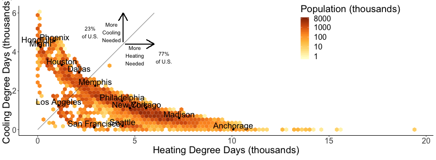
It can be a little hard to see the city names. Looking for a more clear figure or curious where your city falls in cooling and heating degree space?
Check out the interactive version of the above chart here
It’s hard to be a street tree UrbanTrees
Early monocultures and early polycultures. UrbanTrees
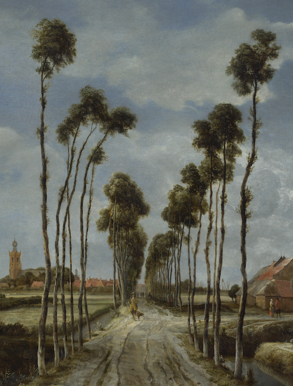
People have liked streets lined with a single species for quite a while. The Roads Beautifying Association observed in 1930:
How the landscape can be transfigured is seen by Hobbema’s painting, which has been one of the world’s favourites for more than two hundred years, “The Avenue at Middelharnis, Holland.”
citep:roads_1930
I had long thought that those who planted trees along streets back in the day only considered planting monocultures. Indeed, many authors take it as a given that this is the preferred, more beautiful way. Only recently with the repeated loss of popular species did I think this idea was being commonly challenged and even then, there are many who prefer monocultures for ease of management. Then I found this article from volume 8 of Scientific American, 1852, and I realized that the desire for a diverse street goes way back.

The article was mostly about the merits and demerits of ailanthus, which was starting to go out of fashion, but there was also this paragraph (emphasis mine):
Our people are too liable to go everything by fashionable excitements, instead of individual independent taste. This is the reason why whole avenues of one kind of tree may be seen in one place, and whole avenues of a different kind in another place; and how at one time one kind of tree, only, will be in demand, and at another period a different tree will be the only one in demand. We like to see variety; and the ailanthus is a beautiful, suitable, and excellent tree to give a chequered air of beauty to the scene. We do not like to see any street lined and shaded with only one kind of tree; we like to see the maple, whitewood, mountain ash, horse-chestnut, ailanthus, &c., mingled in harmonious rows.
It’s an interesting list of species too. I’m not sure what whitewood is, maybe Tilia? Moutain ash, horse-chestnut, and ailanthus are still around but rarely planted as street trees.
update:
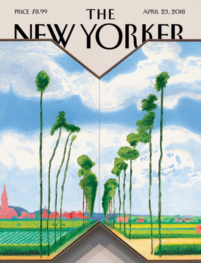
Crazy coincidence that the New Yorker’s April 2018 cover is based on a work by David Hockney which is based on the “Avenue at Middelharnis”.
Street Tree History Time Warp UrbanTrees
I was reading a paper about the susceptibility of urban forests to the emerald ash borer cite:ball_e_2007, when I came across a citation from 1911:
Unfortunately, there are a limited number of tree species adapted to the harsh growing conditions found in many cities, a fact lamented early in the last century (Solotaroff 1911) and repeated to the present day.
After reading this I immediately had the desire to cite somebody from over 100 years ago. Like the author who pulls quotes from Horace to show our unchanging human condition across millennia, I wanted to find my Odes so that I could uncover the ancients’ connection to city trees and determine if it was like my own. How did they view their trees and are we different today?
And then I went down a little history rabbit hole.
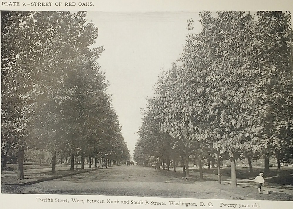
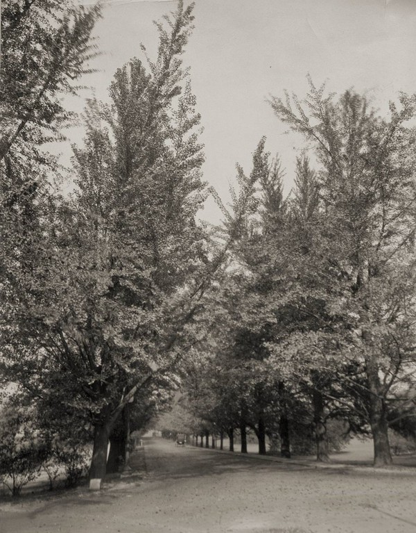
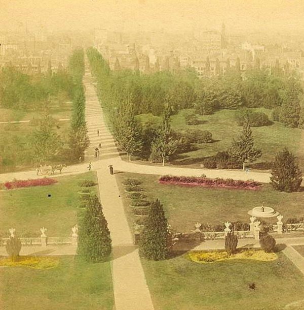
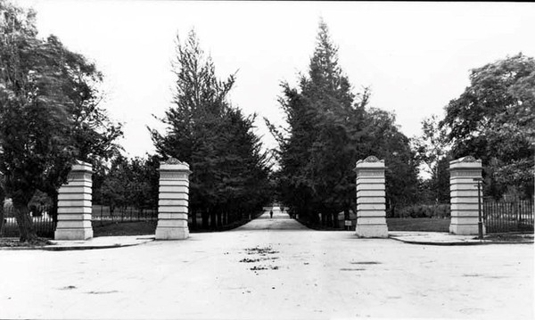
I checked out cite:solotaroff_1911 from the library and quickly realized how some things have changed enormously (public enemy number one of street trees is no longer the horse), while others (the trees themselves) are the same. The book is filled with great photos of tree lined streets, meant to exemplify the beauty of a monospecific street and highlight each species’ characteristics (Figure 29).
I searched for these streets on google street view, to see if the trees survived the century. The few streets I checked before becoming discouraged were radically transformed and the trees were gone. Most had changed with development. Some were located on what would become the national mall and McMillan’s plan removed them. However, with gingkos I did have luck.
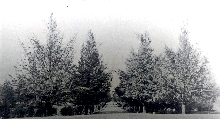
Figure 30 from Solotaroff shows a block of 30 year old gingkos.
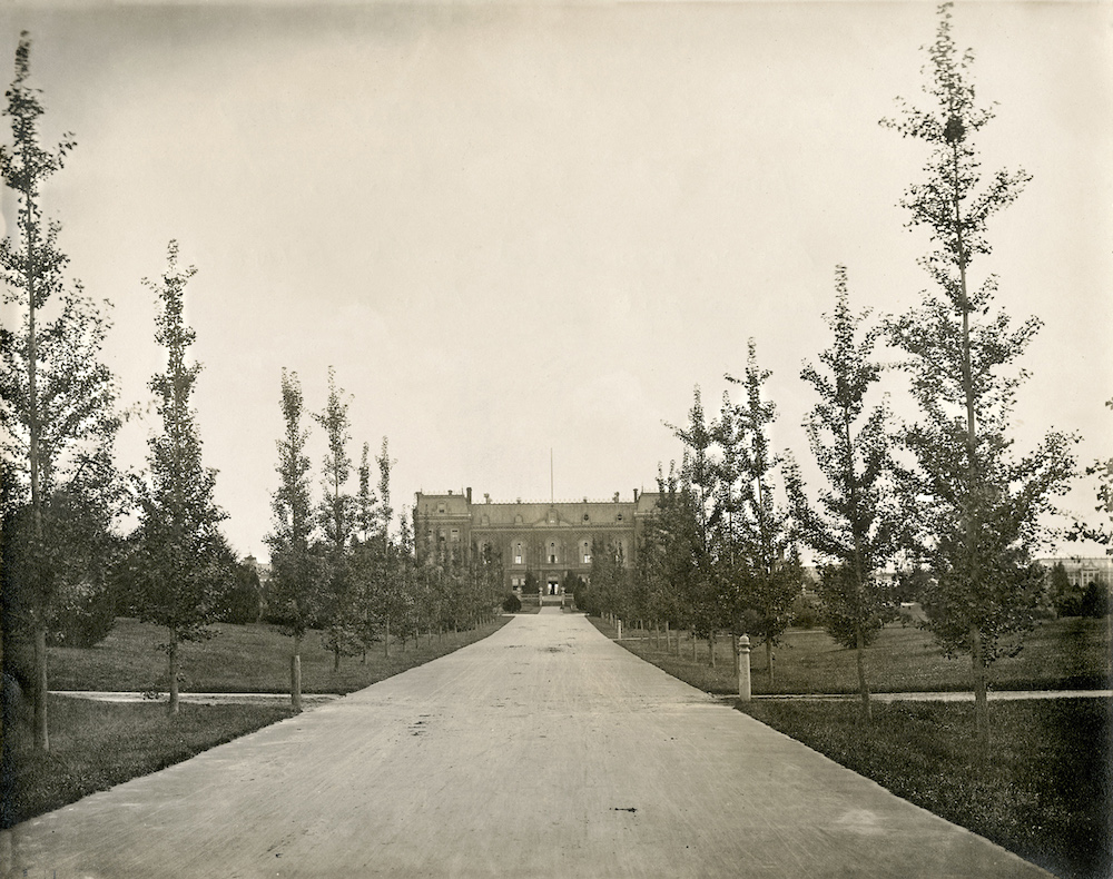
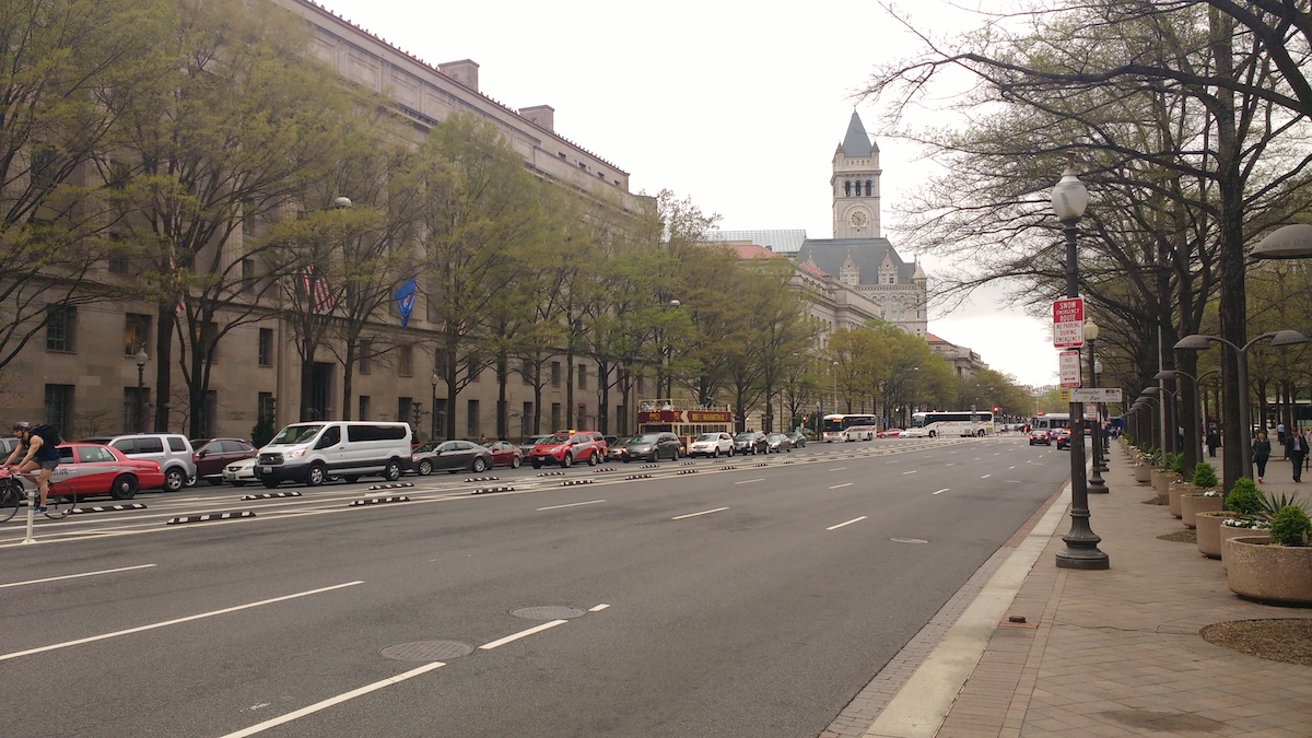
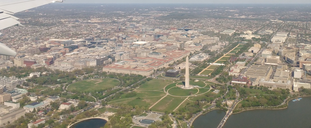
With some searching, I found this article about George Saunders on the USDA website. Saunders was responsible for the planting of the gingkos around 1870 (Figure 31). I also found two photos (I think taken from the Washington Monument), overlooking the mall in 1901 and 1908 in which the ginkgos are visible (Figures 32 and 33). Today, even though the USDA building is now gone, two of the original trees are still around (Figure 34).
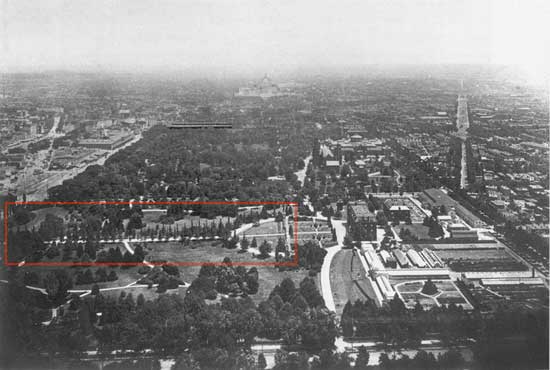
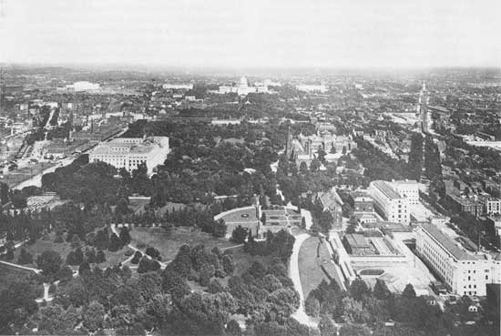
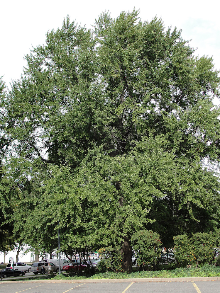
They are a little bit of living history. Their survival to a mature age in such a large city certainly required a lot of people making decisions to spare them during development. Next time I go to D.C. I have a scavenger hunt planned out to see if any of the other trees Solotaroff photographed in 1911 are still around today, or if the only survivor is the hearty ginkgo.
Update
Rob Griesbach at the USDA sent me these additonal photos of the ginkgos:
Thanks, Rob!
NASA Biodiversity and Ecological Forecasting 2018 nasa travel
Team Meeting

Constrained regression for better tree growth equations UrbanTrees
Say you plant a tree in a city. How big will it be in 20 years? You might want to know because the ecosystem services provided by trees is largely a function of their size - the amount of carbon stored in their wood, the amount of shade and evapotranspiration providing cooling, the amount of leaf area reducing sound and air pollution.
The Forest Service’s urban tree database and allometric equations provides equations to predict how tree size changes with age for the purpose of quantifying ecosystem services. These equations are empirical, that is to say, the researchers tested a bunch of equations of different forms (linear, quadratic, cubic, log-log, …) and then selected the form that had the best fit (lowest AIC). What is nice about this method is that provides a good fit for the data. But they don’t take into account knowledge we have about how trees grow, and they could end up making poor predictions on new observations, especially if extrapolated. Here’s an illustration of that problem:
Below is the quadratic function to predict diameter at breast height (DBH) from age.
\[ DBH = a(Age^2) + b(Age) + c + \epsilon \]
where ε is the error term.
See the best fitting quadratic relationship between age and DBH for Tilia americana below. This quadratic function does a good job describing how dbh changes with age (better than any other form they tested).
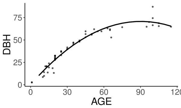
They found the quadratic curve gave the best fit, but unfortunately the curve predicts that DBH begins declining at old age, something we know isn’t true. Diameter should increase monotonically with age. The trouble is that for old trees, the number of samples is small and the variance/error is large. A small random sample can cause the best fitting curve to be decreasing, when we know that if we had more data this wouldn’t be the case. If we constrain the curve to be non decreasing over the range of the data, we can be almost certain to decrease the prediction error for new data.
How to do this?
We need the curve to be monotonically increasing over the range of our data. Or, put another way, we need the x-intercept of the line of symmetry of the quadratic function to be greater than the maximum value of our x data. The line of symmetry is \(x = \frac{-b}{2a}\). We need this to be greater than the maximum value of \(x\)
\[ \frac{-b}{2a} > \max(x) \]
or equivalently
\[ 2a\max(x) + b < 0 \]
The function lsei in the R package limSolve uses quadratic
programming to find the solution that minimizes the sum of squared
error subject to the constraint. I don’t know the math behind this,
but it is very neat. This stats.stackoverflow question and the
limSolve vignette helped me figure this out.
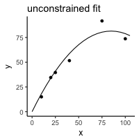
Here is a toy example:
  y <- c(15, 34.5, 39.6, 51.6, 91.7, 73.7)
  x <- c(10L, 20L, 25L, 40L, 75L, 100L)

  a <- data.frame(y = y, x = x)

  m <- lm(y ~ x + I(x^2) - 1)

  p <- data.frame(x = seq(0,105, 5))

  p$y <- predict(m, p)
library(ggplot2)
theme_set(theme_classic(base_size = 12))
ggplot(a, aes(x = x, y = y))  +
geom_point() +
geom_line(data = p) +
ggtitle("unconstrained fit")
  library(limSolve)

  maxx <- max(x)

  A <- matrix(ncol = 2, c(x, x^2))
  B <- y
  G <- matrix(nrow = 1, ncol = 2, byrow = T, data = c(1,2*maxx))  # here's the inequality constriant
  H <- c(0)

  constrained_model <- lsei(A = A,B = B, G = G, H = H, type = 2)

  my_predict <- function(x,coefficients){
      X <- cbind(x,x^2)
      predictions <- X%*%coefficients
  }

                                          # compute predictions
  xpred <- seq(0,105,5)
  predictions_constrained <- my_predict(xpred,constrained_model$X)
  df2 <- data.frame(xpred,predictions_constrained)
theme_set(theme_classic(base_size = 12))
  ggplot(a, aes(x = x, y = y))  +
  geom_point() +
  geom_line(data = df2, aes(x = xpred, y = predictions_constrained)) +
ggtitle("constrained")

The constrained curve looks pretty good.
Just a quick note about using lsei, the signs are not what I
expected them to be in the G matrix. Maybe my math is wrong somewhere
or I don’t fully understand the limSolve package. According to my
equation above the G matrix should have negative values, but the
solution is correct, so I’m going to go with that. If you read this
and find my error, please tell me.
Even after constraining the quadratic curve to be increasing over the range of data, it’s still not ideal. Extrapolation will certainly give bad predictions because the curve begins decreasing. The quadratic curve is nice because it is simple and easy and fits the data well, but it is probably better to select a model form that is grounded in the extensive knowledge we have of how trees grow. The goal of the urban tree database to create equations specific to urban trees which may have different growth parameters than trees found in forests. But the basic physiology governing tree growth is the same regardless of where the tree is growing, and it makes sense to use a model form that considers this physiology, like something from here.
Even if I won’t use this, I’m happy to have learned how to perform a regression with a somewhat complex constraint on the parameters.
Update: I found out QP is a pretty standard thing in linear algebra and that it’s used to connect splines. Neat.
Commuting Across Mendota life
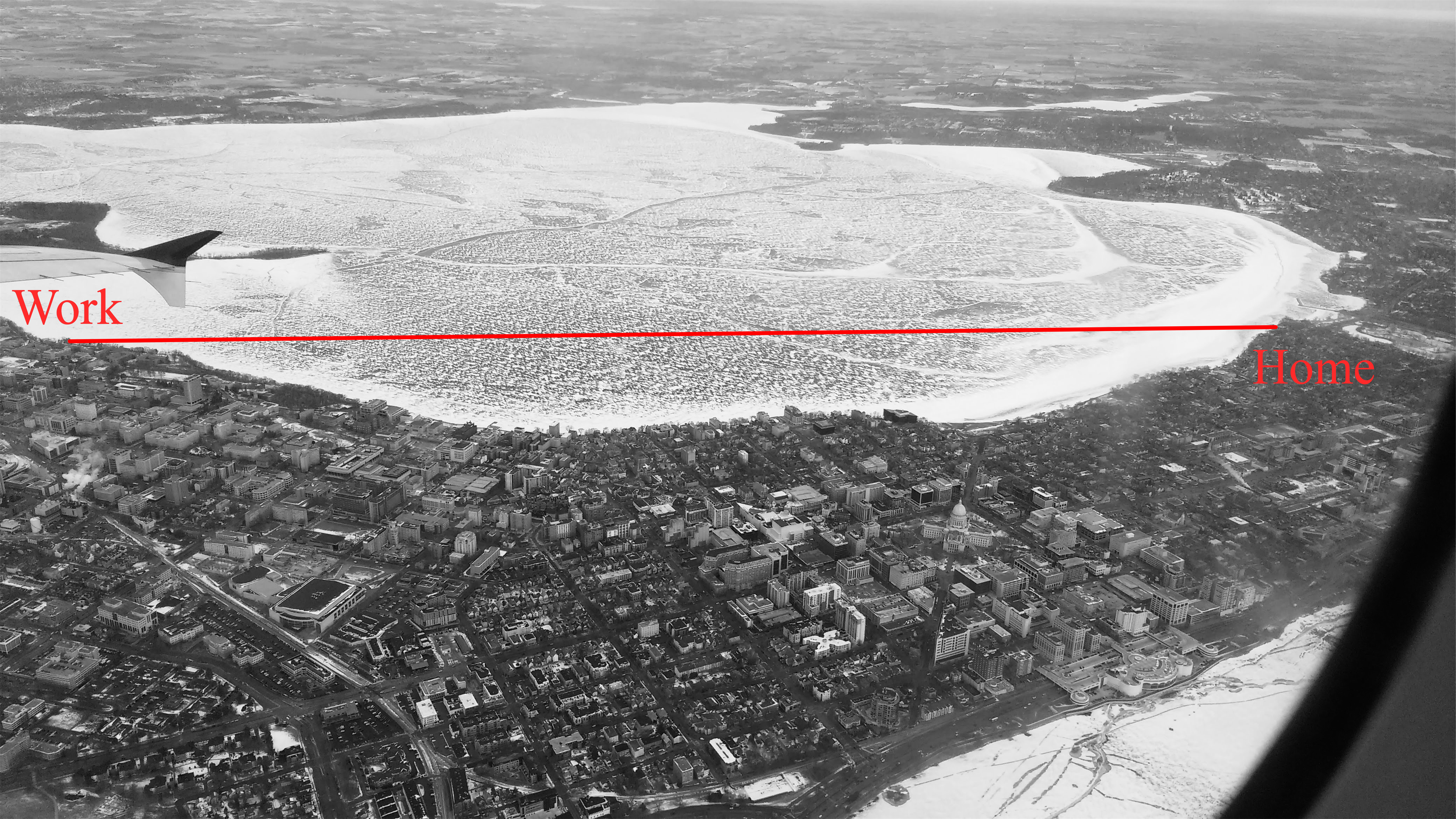


The best way to get to work is by ice.
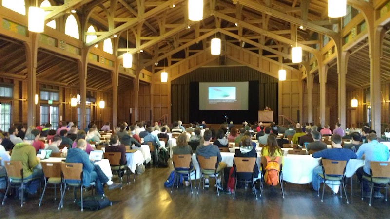
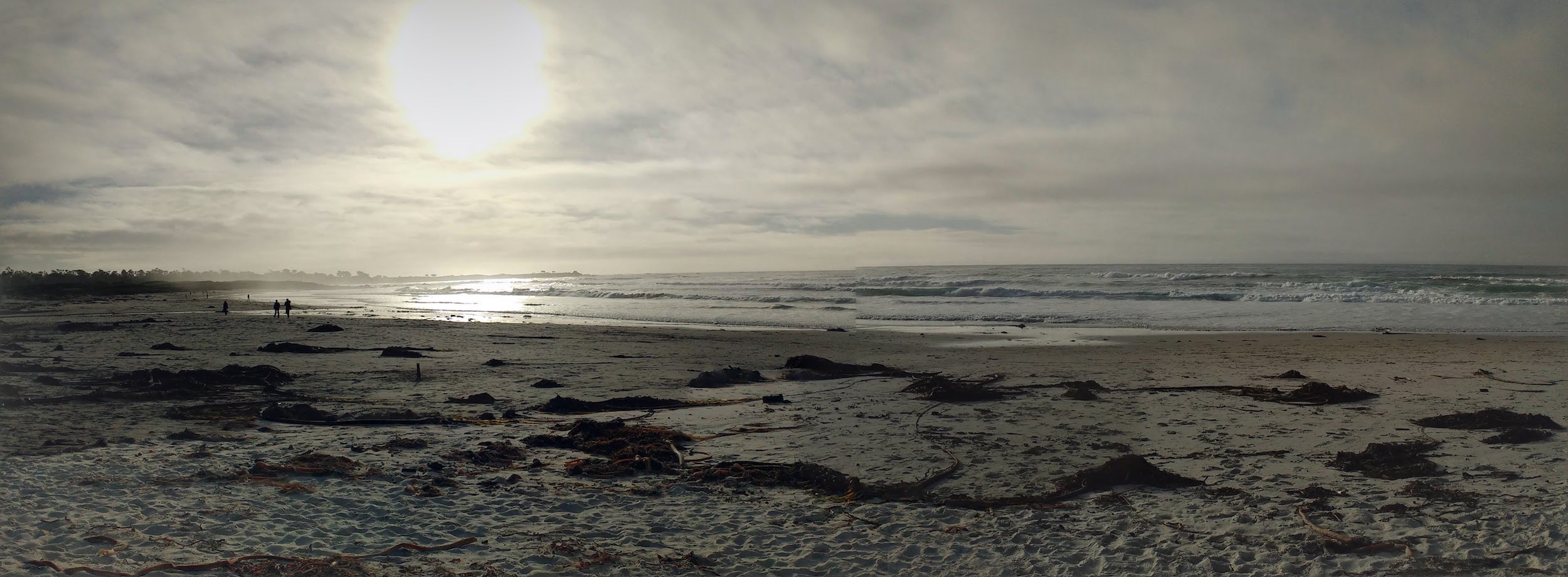
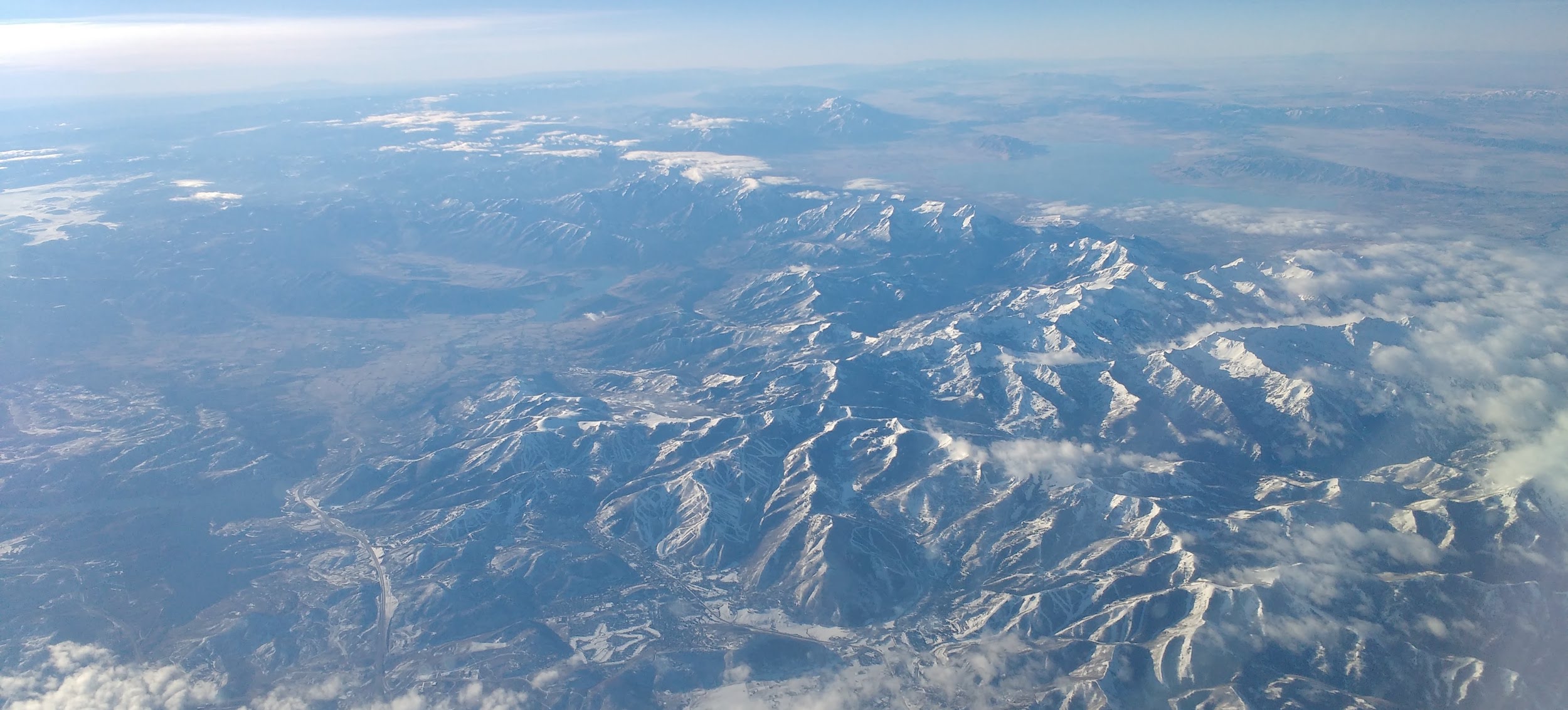
STANCon 2018 statistics
Stan is a probabilistic programming language used for bayesian statistical inference. I got a student scholarship to attend the Stan conference 2018 in Monterey this January.
The view from an airplane is always amazing:


My personal highlight of the conference was meeting and chatting with other attendees at family style meals. It is truly amazing the variety of fields in which Stan is used. I had many productive and enlightening conversations.
Here are few more quick take-aways:
- R packages rstanarm and brms can help you fit Stan models using R syntax many people may be more comfortable with, such as the lme4 syntax for multilevel models. They can also output the stan code for tweaking.
- Fitting customized hierarchical models can be challenging in Stan for a non expert like me. But the flexibility of these models is attractive.
- The regularized horseshoe prior is an option for shrinking parameter estimates. I’d like to test it out for some of the problems our lab faces. I don’t think it would provide predictive improvements, but it might enhance inference by identifying important variables.
- “Our work is unimportant.” Andrew Gelman, the lead of the Stan team and final speaker, emphasized this point, that bayesian inference hasn’t done much for humanity. It was a humbling and thought-provoking comment to end three days of talking about all the things that we use Stan for. It was a good point for reflection and a reminder that I need to balance my compulsions to do technically correct/advanced/obtuse science with my desire to do science that actually gets done and contributes to society.
- Gelman also mentioned that our work can be like a ladder: Scientists must become statisticians to do science, statisticians must become computational statisticians to do statistics, computational statisticians must become software developers … and so on. As a scientist who constantly feels like he’s in over his head with statistics, I appreciated this point. To achieve our objectives we must stretch ourselves. It’s never comfortable to feel like we don’t know what we are doing, but how else can we grow?
It was also very beautiful there:
Statistics and Elections statistics
Statistics can be a powerful tool for identifying fraud in elections. One of my favorite examples comes from the 2011 Russian election. See the wikipedia article and this figure. The distribution of the votes has very abnormal peaks at every 5%.
The Honduran election that just happened is also suspect to fraud and the economist did a quick analysis to test for any sign of interference in the voting. Check out their article here for the details. But the gist of their work investigates changes in the distribution of voting from one day to the next, with the premise being that Hernández’s party saw they were losing and stuffed the ballots near the end of voting. I’m curious to see what comes of this. To me it seems like a recount is in order.
Thank you statistics.
UPDATE
Maybe statistics is not that helpful. The U.S. recognizes Hernández as president despite the irregularities. See the wikipedia article. Perhaps statistics can identify a problem with a certain level of confidence, but it cannot solve that problem. These two cases are disappointing, and I’m curious if there are elections where fraud was identified with statistics and this revelation led to a redo.
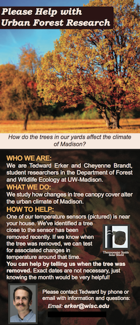
(Not) Remembering When Trees Disappear
One of the fun parts of my work this semester was knocking on doors and asking people when nearby trees were removed. We wanted to see if the removal of the trees affected the area’s air temperature. The residents were super helpful and many gave us very precise and accurate dates for when trees were removed, especially for trees from their own yards. However, many were not sure about street tree removals and so we double checked dates with city Forester’s records. (A big thanks goes to to Robi Phetteplace, Marla Eddy and Brittany Prosser for helping with this!) When I did the double checking, I was surprised at how far off many of the resident’s guesses were. Below is a table which shows that a resident’s best guess of when a street tree was removed is usually off by several months, even when the removal happened recently.
| Residents Best Guess | Forester Records Show | Difference (apprx) |
|---|---|---|
| sep 2017 | 2017-07-12 | 2 months |
| sep 2017 | 2017-06-20 | 2-3 months |
| fall 2016 | 2016-06-30 | 3-4 months |
| didn’t think tree ever existed | 2016 spring | |
| spring 2017 | 2016-03-15 | 1 year |
| before june 2015 | 2015-10-02 | 4 months |
| 2016 | 2015-04-02 | 6 months |
| fall 2015 | 2015-01-09 | 9-11 months |
Probably most surprising was a resident who, when asked about a tree, said that no tree ever existed there.
On the other side of the memory spectrum, there was one resident, Sara S, who could exactly date when a tree was removed because she had photo evidence and a good story. Minutes before a hail storm blew through, she told her daughter to move her car inside. Shortly after, the tree the car was parked under split in half. It was removed the next day.
I think the insight to be gained from these informal observations is that people don’t remember things unless they are important to them. Even though we see these trees everyday, they aren’t important enough for us to remember when they go away. But I’m not judging, I can’t even remember my good friend’s birthdays, so why should I expect people to be able to recall when a tree was removed?
Our memories just aren’t so good, and it’s important to remember that when doing research.
Flyer to get citizen help with urban forest research. UrbanHeatIsland
 |
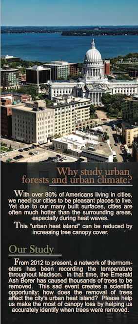 |
This is a beautiful flyer created by Cheyenne to leave on the doors of houses who don’t answer when we knock to find out when a nearby tree was removed. As of today we’ve had a couple responses that have given us the exact date trees were removed. Thank you Sara Sandberg and Mike Bussan!
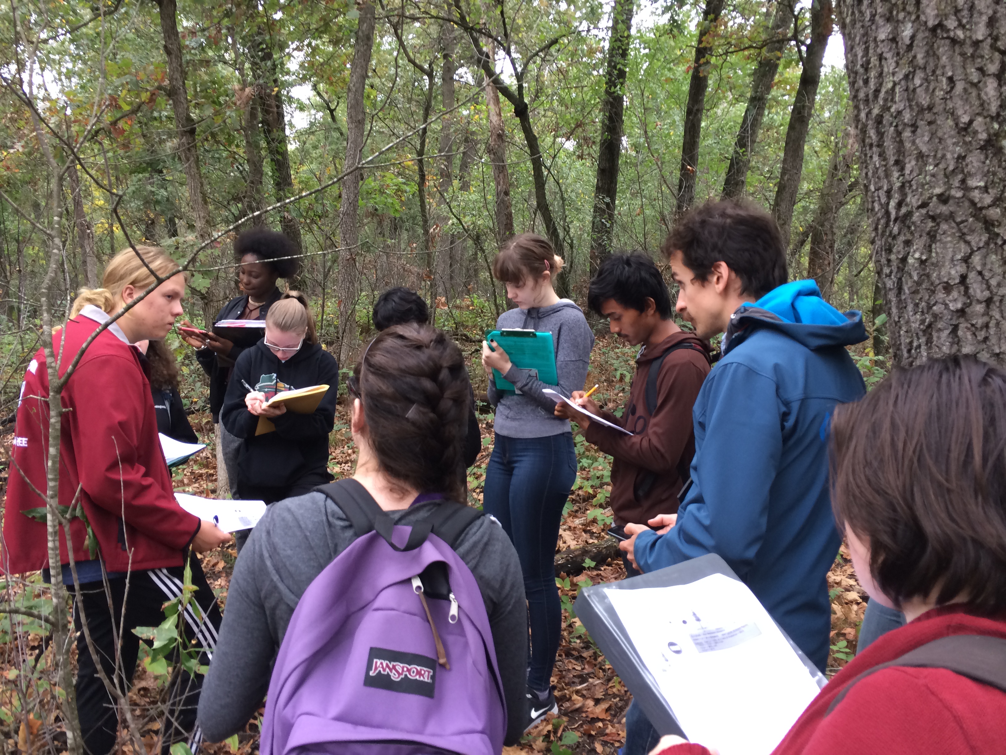
Madison East AP Environmental Studies Field Trip
I got to help students in Madison East’s AP Environmental studies on their field trip to the Madison School Forest. With 85 students and just one teacher, it was a big undertaking, but their teacher, Angie Wilcox-Hull, did an awesome job organizing.
They learned how identify common Wisconsin tree species and also did a lab on carbon in forests. Students used a clinometer and diameter at breast height tape to measure forest trees, they estimated carbon content of the trees, and they compared this to the carbon emissions caused by their transportation to and from school. As always it was great to work with high school students and there were a lot of great questions and points brought up. Here are four that were especially salient to me:
- Students realized that we used the equation of a cylindar to approximate the volume of a tree, but a cone is usually more appropriate.
- When we talked about finding the volume of wood in leaning trees, one student used his knowledge of calculus to tell me it wasn’t quite so hard. See here. I wonder if foresters use that idea for leaning trees.
- Carbon storage is not the same as carbon sequestration
- While we measured individual trees, carbon stored per area of land may be more interesting for managers.
Second Trip to Washington, DC for NASA’s Biodiversity and Ecological Forecasting Team Meeting nasa travel

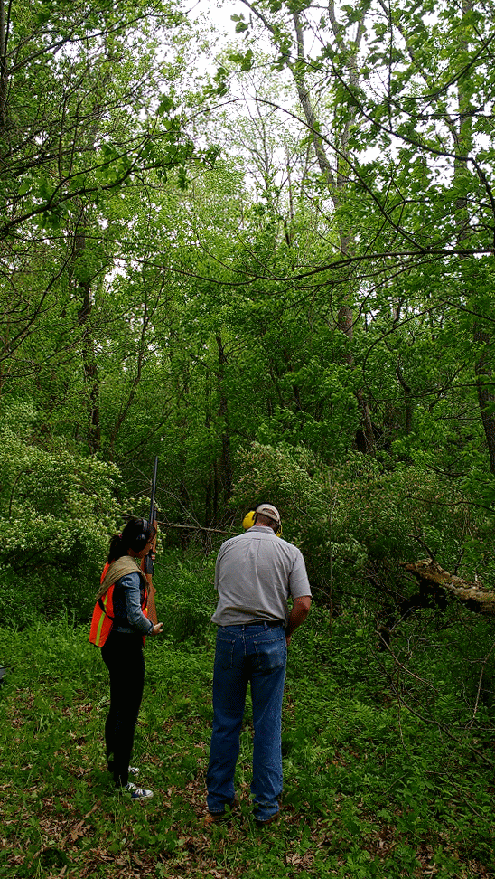
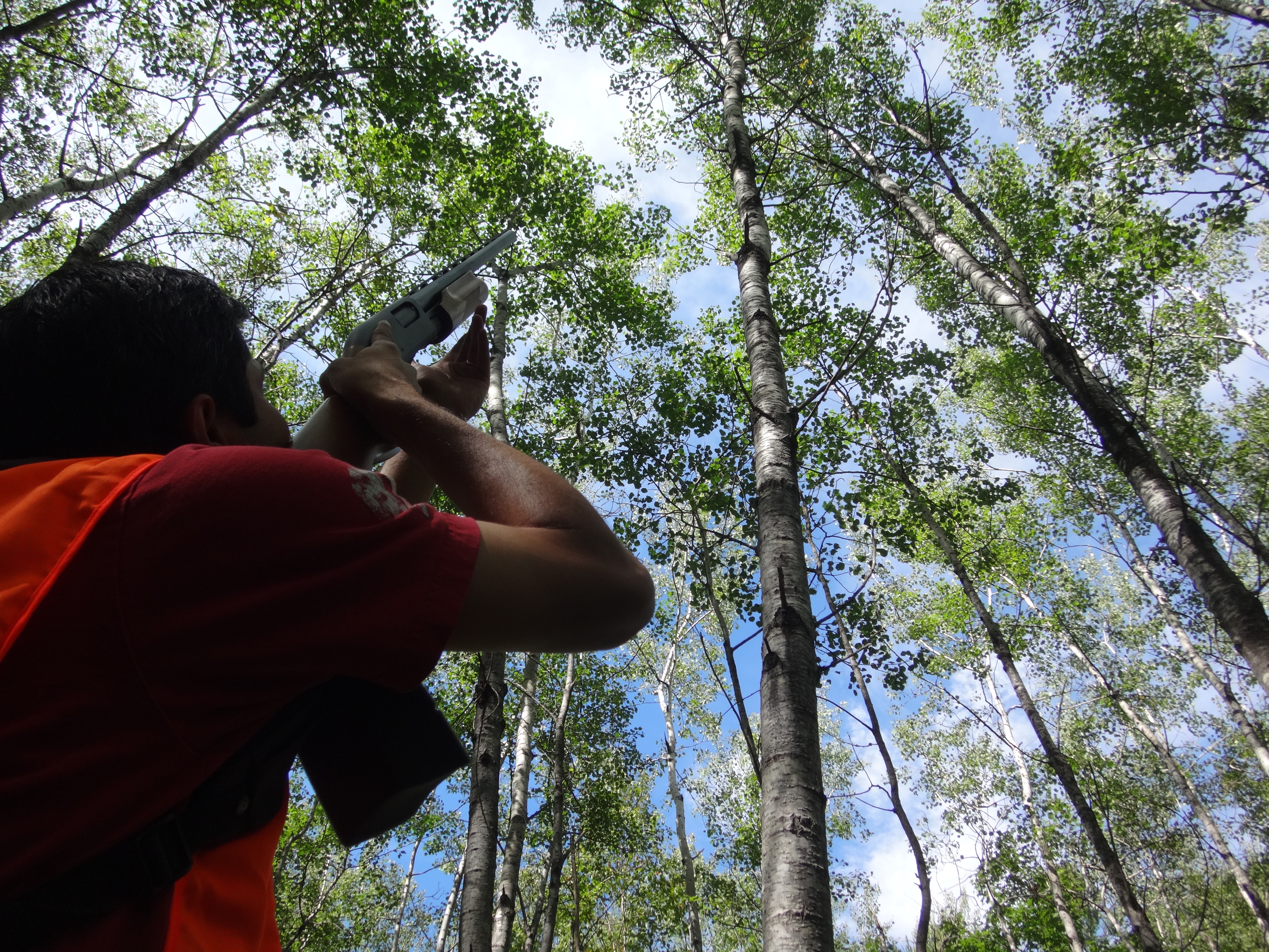
Shotgun Training
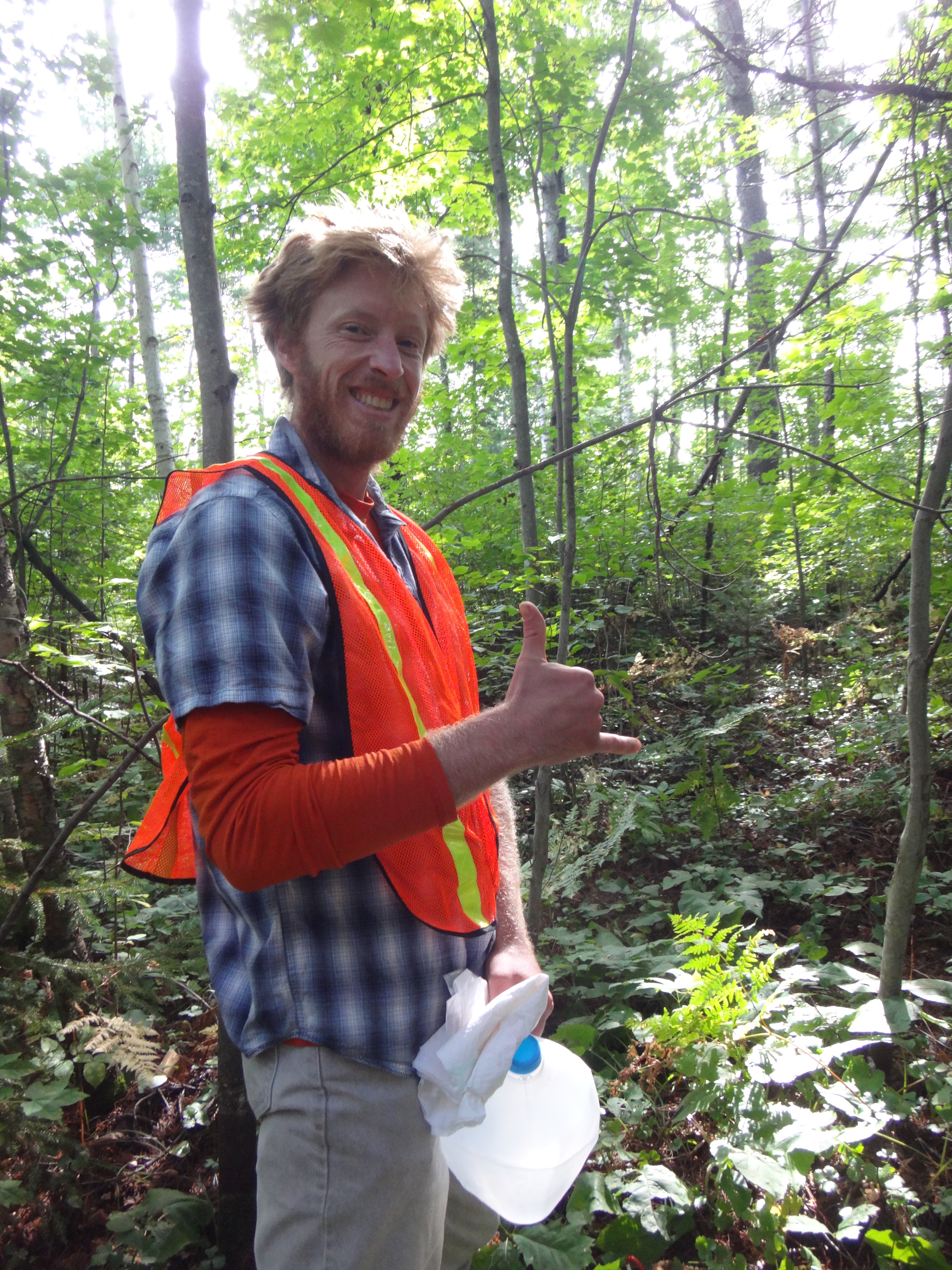
Collecting Urban Heat Island Data with Carly Ziter UrbanHeatIsland
Using OpenBLAS to speed up matrix operations in R (linux) computing
I use the foreach and doParallel packages in R to speed up my work
that can be easily parallelized. However, sometimes work can’t be
easily parallelized and things are slower than I’d like. An example
of this might be fitting a single very large and complex model. Andy
Finley, who resently stopped by UW-Madison to give a workshop on
hierarchical modeling, taught us about OpenBLAS as a way to speed up
matrix operations in R. Here are the notes about computing from the
workshop.
BLAS is Basic Linear Algebra Subprograms. R and other higher level languages call BLAS to do matrix operations. There are other versions of BLAS, such as OpenBLAS, which are faster than the default BLAS that comes with R because they are able to take advantage of multiple cores in a machine. This is the extent of my knowledge on the topic.
Below is how I installed OpenBLAS locally on our linux server and pointed R to use the OpenBLAS instead of its default BLAS. A benchmark test follows.
Getting OpenBLAS
cd src                         # move to src directory to download source code
wget http://github.com/xianyi/OpenBLAS/archive/v0.2.19.tar.gz    # your version may be different
tar xzf v0.2.19.tar.gz
cd OpenBLAS-0.2.19/
make clean
make USE_OPENMP=1               #OPENMP is a threading library recommended by Andy Finley
mkdir /home/erker/local
make PREFIX=/home/erker/local install       # You will have to change your install location
Pointing R to use OpenBLAS
I have R installed in my ~/local directory. libRblas.so is the default
BLAS that comes with R. For me it is located in ~/local/lib/R/lib.
Getting R to use OpenBLAS is as simple as changing the name of the
default BLAS and creating a link in its place that points to OpenBLAS:
  mv libRblas.so libRblas_default.so
  ln -s ~/local/lib/libopenblas.so libRblas.so
Deleting the link and reverting the name of the default BLAS, will make R use the default BLAS again. Something like:
  rm libRblas.so
  mv libRblas_default.so libRblas.so
Benchmark Test
I copied how to do this benchmark test from here. The benchmark test time was cut from about 146 to about 38 seconds on our server. This is a very significant speed up. Thank you OpenBLAS and Andy Finley.
- Default BLAS
  curl http://r.research.att.com/benchmarks/R-benchmark-25.R -O
  cat R-benchmark-25.R | time R --slave
Loading required package: Matrix Loading required package: SuppDists Warning messages: 1: In remove("a", "b") : object 'a' not found 2: In remove("a", "b") : object 'b' not found R Benchmark 2.5 =============== Number of times each test is run__________________________: 3 I. Matrix calculation --------------------- Creation, transp., deformation of a 2500x2500 matrix (sec): 0.671333333333333 2400x2400 normal distributed random matrix ^1000____ (sec): 0.499666666666667 Sorting of 7,000,000 random values__________________ (sec): 0.701666666666667 2800x2800 cross-product matrix (b = a' * a)_________ (sec): 10.408 Linear regr. over a 3000x3000 matrix (c = a \ b')___ (sec): 4.877 -------------------------------------------- Trimmed geom. mean (2 extremes eliminated): 1.31949354763381 II. Matrix functions -------------------- FFT over 2,400,000 random values____________________ (sec): 0.220333333333334 Eigenvalues of a 640x640 random matrix______________ (sec): 0.717666666666664 Determinant of a 2500x2500 random matrix____________ (sec): 3.127 Cholesky decomposition of a 3000x3000 matrix________ (sec): 4.15 Inverse of a 1600x1600 random matrix________________ (sec): 2.364 -------------------------------------------- Trimmed geom. mean (2 extremes eliminated): 1.74407855808281 III. Programmation ------------------ 3,500,000 Fibonacci numbers calculation (vector calc)(sec): 0.503999999999981 Creation of a 3000x3000 Hilbert matrix (matrix calc) (sec): 0.259999999999991 Grand common divisors of 400,000 pairs (recursion)__ (sec): 0.301000000000007 Creation of a 500x500 Toeplitz matrix (loops)_______ (sec): 0.0393333333333317 Escoufier's method on a 45x45 matrix (mixed)________ (sec): 0.305999999999983 -------------------------------------------- Trimmed geom. mean (2 extremes eliminated): 0.288239673174189 Total time for all 15 tests_________________________ (sec): 29.147 Overall mean (sum of I, II and III trimmed means/3)_ (sec): 0.87211888350174 --- End of test --- 144.64user 0.94system 2:25.59elapsed 99%CPU (0avgtext+0avgdata 454464maxresident)k 0inputs+0outputs (0major+290577minor)pagefaults 0swaps - OpenBLAS
cat R-benchmark-25.R | time R --slave
Loading required package: Matrix
Loading required package: SuppDists
Warning messages:
1: In remove("a", "b") : object 'a' not found
2: In remove("a", "b") : object 'b' not found


R Benchmark 2.5
===============
Number of times each test is run__________________________:  3

I. Matrix calculation
---------------------
Creation, transp., deformation of a 2500x2500 matrix (sec):  0.689666666666667
2400x2400 normal distributed random matrix ^1000____ (sec):  0.499
Sorting of 7,000,000 random values__________________ (sec):  0.701
2800x2800 cross-product matrix (b = a' * a)_________ (sec):  0.163000000000001
Linear regr. over a 3000x3000 matrix (c = a \ b')___ (sec):  0.228
--------------------------------------------
Trimmed geom. mean (2 extremes eliminated):  0.428112796718245

II. Matrix functions
--------------------
FFT over 2,400,000 random values____________________ (sec):  0.224333333333332
Eigenvalues of a 640x640 random matrix______________ (sec):  1.35366666666667
Determinant of a 2500x2500 random matrix____________ (sec):  0.140666666666667
Cholesky decomposition of a 3000x3000 matrix________ (sec):  0.280333333333332
Inverse of a 1600x1600 random matrix________________ (sec):  0.247000000000001
--------------------------------------------
Trimmed geom. mean (2 extremes eliminated):  0.249510313157146

III. Programmation
------------------
3,500,000 Fibonacci numbers calculation (vector calc)(sec):  0.505000000000001
Creation of a 3000x3000 Hilbert matrix (matrix calc) (sec):  0.259333333333333
Grand common divisors of 400,000 pairs (recursion)__ (sec):  0.299333333333332
Creation of a 500x500 Toeplitz matrix (loops)_______ (sec):  0.039333333333334
Escoufier's method on a 45x45 matrix (mixed)________ (sec):  0.256999999999998
--------------------------------------------
Trimmed geom. mean (2 extremes eliminated):  0.271216130718114


Total time for all 15 tests_________________________ (sec):  5.88666666666666
Overall mean (sum of I, II and III trimmed means/3)_ (sec):  0.30712894095638
--- End of test ---

176.85user 12.20system 0:38.00elapsed 497%CPU (0avgtext+0avgdata 561188maxresident)k
0inputs+0outputs (0major+320321minor)pagefaults 0swaps
Next things
From comments here, I have heard that OpenBLAS doesn’t play well with
foreach and doParallel. I will have to test these next. If it is
an issue, I may have to include a shell code chunk in a literate program
to change between BLAS libraries.
Application Essay: Catalyzing Advocacy in Science and Engineering: 2017 Workshop
I just applied to the CASE 2017 Workshop in Washington, DC. The application process led to some interesting thoughts, so I thought I’d share the essay.
Update : I was not accepted.
Application
“How do we know the earth is 4.5 billion years old?” I loved asking my students this question when I taught high school science. The students (and I) were hard pressed to explain how we know this to be true. Most of us don’t have the time to fully understand radiometric dating, let alone collect our own data from meteorites to verify the earth’s age. So unless it’s a topic we can investigate ourselves, we must simply trust that scientists are following the scientific method and evaluate their results within the context of our own experience.
Trust between scientists and the public is therefore the necessary foundation upon which our society accepts scientific research, incorporates it into policy, and supports more science. The communication of science’s benefits to society maintains this trust. Unfortunately, the public and scientists disagree in many critical areas of research, such as genetic modification, climate change, evolution, vaccinations, and the age of the earth (1) (2). I believe scientists must do more to directly address these discrepancies.
As a scientist I have the incredible opportunity to conduct research that I think will improve society, and I’m honored that the public pays me to do it. I’m making a withdrawal from the bank of public trust and feel strongly that I need to pay it back with interest. I see scientific communication as the way to do so. Effective scientific communication goes way beyond publishing quality work in reputable journals and requires that we place our findings into the public consciousness. I have taught at the university and have led a few guest labs at an area high school, but I want to have a greater impact. The CASE 2017 workshop excites me with the opportunity to learn how to make this impact.
My hope is that CASE will orient me to the landscape of science advocacy, policy, and communication. Despite benefiting from federal funds for science, I am mostly ignorant of how our nation allocates resources to research, and I look forward to CASE demystifying this process. I hope to learn effective methods to communicate science with the public and to discuss with elected officials the value of research for crafting smart policy.
Because scientists understand their work best, they are best suited to advocate for it. CASE will provide a unique opportunity to learn how to be an advocate for science and a leader in strengthening the trust between the scientific community and the public whom we serve. If selected, I would like to work with the other selected graduate student and the graduate school’s office of professional development to host a mini-workshop to bring the knowledge and skills from CASE to our campus. I’d like to replicate the Capitol Hill visits at a state level and work to get more graduate students engaged with elected officials from across the state.
OBSOLETE:Installing R, gdal, geos, and proj4 on UW Madison’s Center for High Throughput Computing computing
NOTE
This post is obsolete. Use Docker as the chtc website now recommends
R is the language I use most often for my work. The spatial packages of R that I use very frequently like rgdal, rgeos, and gdalUtils depend on external software, namely gdal, proj4, and geos.
Here I show how I installed gdal, proj4, and geos on chtc, and pointed the R packages to these so that they install correctly.
The R part of this tutorial comes from chtc’s website. Their site should be considered authoritative. I quote them heavily below. My effort here is to help people in the future (including myself) to install gdal etc. on chtc.
Create the interactive submit file. Mine is called interactive_BuildR.sub
I save it in a directory called “Learn_CHTC”
  universe = vanilla
  # Name the log file:
  log = interactive.log

  # Name the files where standard output and error should be saved:
  output = process.out
  error = process.err

  # If you wish to compile code, you'll need the below lines.
  #  Otherwise, LEAVE THEM OUT if you just want to interactively test!
  +IsBuildJob = true
  requirements = (OpSysAndVer =?= "SL6") && ( IsBuildSlot == true )

  # Indicate all files that need to go into the interactive job session,
  #  including any tar files that you prepared:
  # transfer_input_files = R-3.2.5.tar.gz, gdal.tar.gz
  # I comment out the transfer_input_files line because I download tar.gz's from compute node

  # It's still important to request enough computing resources. The below
  #  values are a good starting point, but consider your file sizes for an
  #  estimate of "disk" and use any other information you might have
  #  for "memory" and/or "cpus".
  request_cpus = 1
  request_memory = 1GB
  request_disk = 1GB

  queue
transfer interactive submit file to condor submit node
change erker to your username and if you don’t use submit-3, change
that too. You’ll have to be inside the directory that contains
“interactive_BuildR.sub” for this to work.
rsync -avz interactive_BuildR.sub erker@submit-3.chtc.wisc.edu:~/
log into submit node and submit job
ssh submit-3.chtc.wisc.edu
condor_submit -i interactive_BuildR.sub
wait for job to start
Installing GDAL, Proj4, Geos
Each install is slightly different, but follows the same pattern. This worked for me on this date, but may not work in the future.
- GDAL: Download, configure, make, make install gdal, then tar it up
  wget http://download.osgeo.org/gdal/gdal-1.9.2.tar.gz # download gdal tarball
  tar -xzf gdal-1.9.2.tar.gz # unzip it
  mkdir gdal # create a directory to install gdal into
  dir_for_build=$(pwd) # create a variable to indicate this directory (gdal doesn't like relative paths)
  cd gdal-1.9.2 # go into the unzipped gdal directory
  ./autogen.sh # run autogen.sh
  ./configure --prefix=$dir_for_build/gdal # run configure, pointing gdal to be installed in the directory you just created (You'll have to change the path)
  make
  make install
  cd ..
  tar -czf gdal.tar.gz gdal #zip up your gdal installation to send back and forth between compute and submit nodes
- Proj4: Download, configure, make, make install proj4 then tar it up
  wget https://github.com/OSGeo/proj.4/archive/master.zip
  unzip master.zip
  mkdir proj4
  cd proj.4-master
  ./autogen.sh
  ./configure --prefix=$dir_for_build/proj4
  make
  make install
  cd ..
  tar -czf proj4.tar.gz proj4
- Geos:
  wget http://download.osgeo.org/geos/geos-3.6.0.tar.bz2
  tar -xjf geos-3.6.0.tar.bz2 # need to use the "j" argumnet because .bz2 not gz
  mkdir geos
  cd geos-3.6.0
  ./configure --prefix=$dir_for_build/geos # no autogen.sh
  make
  make install
  cd ..
  tar -czf geos.tar.gz geos
Add libs to LD_LIBRARY_PATH
I don’t actually know what this path is exactly, but adding gdal/lib,
proj4/lib, and geos/lib to the LD_LIBRARY_PATH resolved errors I had
related to files not being found when installing in R. For rgdal the error was
  Error in dyn.load(file, DLLpath = DLLpath, ...) :
  unable to load shared object '/home/erker/R-3.2.5/library/rgdal/libs/rgdal.
and lines like this:
...
./proj_conf_test: error while loading shared libraries: libproj.so.12: cannot open shared object file: No such file or directory
...
proj_conf_test.c:3: error: conflicting types for 'pj_open_lib'
/home/erker/proj4/include/proj_api.h:169: note: previous declaration of 'pj_open_lib' was here
./proj_conf_test: error while loading shared libraries: libproj.so.12: cannot open shared object file: No such file or directory
...
For rgeos the error was
"configure: error: cannot run C compiled programs"
Run this to fix these errors
export LD_LIBRARY_PATH=$LD_LIBRARY_PATH:$(pwd)/gdal/lib:$(pwd)/proj4/lib # this is to install rgdal properly
export LD_LIBRARY_PATH=$LD_LIBRARY_PATH:$(pwd)/geos/lib # and rgeos
If you run:
echo $LD_LIBRARY_PATH
The output should look something like
:/var/lib/condor/execute/slot1/dir_2924969/gdal/lib:/var/lib/condor/execute/slot1/dir_2924969/proj4/lib:/var/lib/condor/execute/slot1/dir_2924969/geos/lib
R: download, untar and move into R source directory, configure, make, make install
As of R 3.3.0 or higher isn’t supported on chtc
    wget https://cran.r-project.org/src/base/R-3/R-3.2.5.tar.gz
    tar -xzf R-3.2.5.tar.gz
    cd R-3.2.5
    ./configure --prefix=$(pwd)
    make
    make install
    cd ..
Install R packages
The installation steps above should have generated an R installation in the lib64 subdirectory of the installation directory. We can start R by typing the path to that installation, like so:
R-3.2.5/lib64/R/bin/R
This should open up an R console, which is how we’re going to install any extra R libraries. Install each of the library packages your code needs by using R’s install.packages command. Use HTTP, not HTTPS for your CRAN mirror. I always download from wustl, my alma mater. For rgdal and rgeos you need to point the package to gdal, proj4 and geos using configure.args
Change your vector of packages according to your needs.
  install.packages('rgdal', type = "source", configure.args=c(
       paste0('--with-gdal-config=',getwd(),'/gdal/bin/gdal-config'),
       paste0('--with-proj-include=',getwd(),'/proj4/include'),
       paste0('--with-proj-lib=',getwd(),'/proj4/lib')))

  install.packages("rgeos", type = "source", configure.args=c(paste0("--with-geos-config=",getwd(),"/geos/bin/geos-config")))

        install.packages(c("gdalUtils",
                           "mlr",
                           "broom",
                           "raster",
                           "plyr",
                           "ggplot2",
                           "dplyr",
                           "tidyr",
                           "stringr",
                           "foreach",
                           "doParallel",
                           "glcm",
                           "randomForest",
                           "kernlab",
                           "irace",
                           "parallelMap",
                           "e1071",
                           "FSelector",
                           "lubridate",
                           "adabag",
                           "gbm"))
Exit R when packages installed
q()
Edit the R executable
nano R-3.2.5/lib64/R/bin/R
The above will open up the main R executable. You will need to change the first line, from something like:
R_HOME_DIR=/var/lib/condor/execute/slot1/dir_554715/R-3.1.0/lib64/R
to
R_HOME_DIR=$(pwd)/R
Save and close the file. (In nano, this will be CTRL-O, followed by CTRL-X.)
Move R installation to main directory and Tar so that it will be returned to submit node
mv R-3.2.5/lib64/R ./
tar -czvf R.tar.gz R/
Exit the interactive job
exit
Upon exiting, the tar.gz files created should be sent back to your submit node
Cool Science Image contest

I created this image of Madison’s lakes using hyperspectral imagery from NASA’s AVIRIS sensor for the Cool Science Image Contest. I threw it together the week before the contest and was very pleased to be selected, but I wish that it had been more related to the science that I do. It is a minimum noise fraction transformation which is a way to transform/condense the data from the ~250 bands into the 3 visible channels (rgb) for maximum information viewing. Originally I intended to create an image over land, but had great difficulty getting the mosaicing of the 3 flightlines to be seamless. You can see the band across the northern part of lake Mendota from fox bluff to warner bay that is due to image processing, not something real in the water. The image is no doubt cool, but I wish I could say more what the colors meant (If you’re a limnologist and see some meaning, please let me know). I think that pink may be related to sand, and green to bright reflections on the water. There’s probably some algae detection going on too. My goal for next year is to make an image that is heavier on the science and still very cool.
Field work in northern Wisconsin
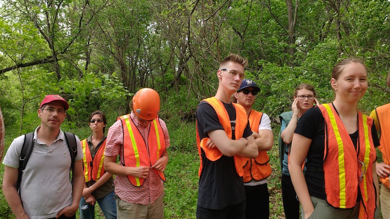
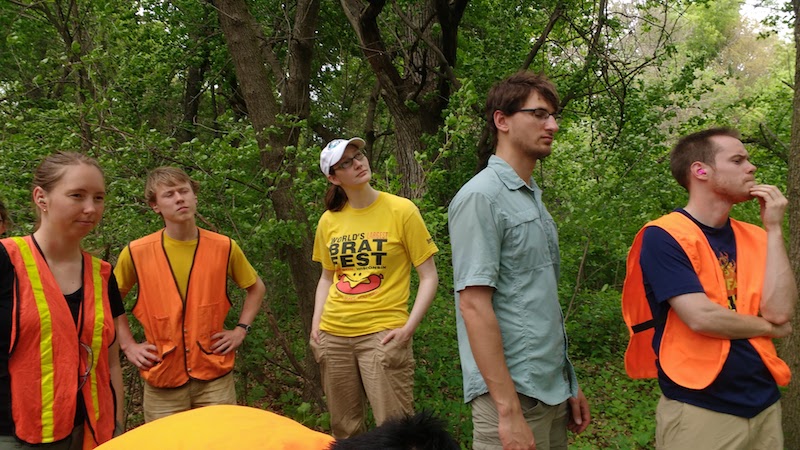
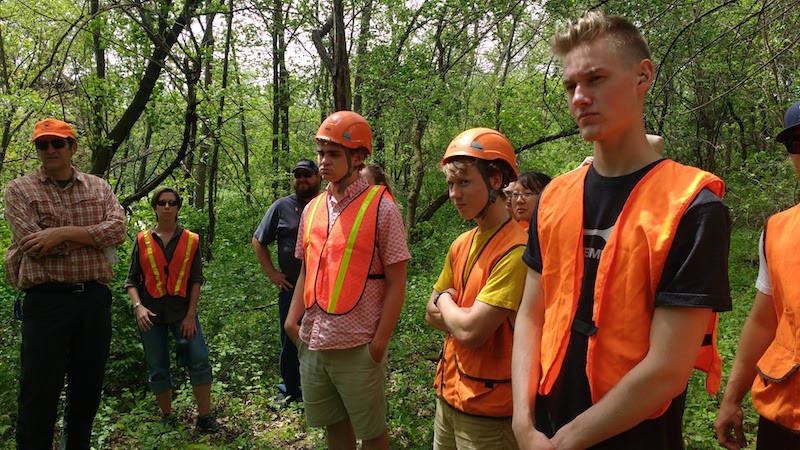
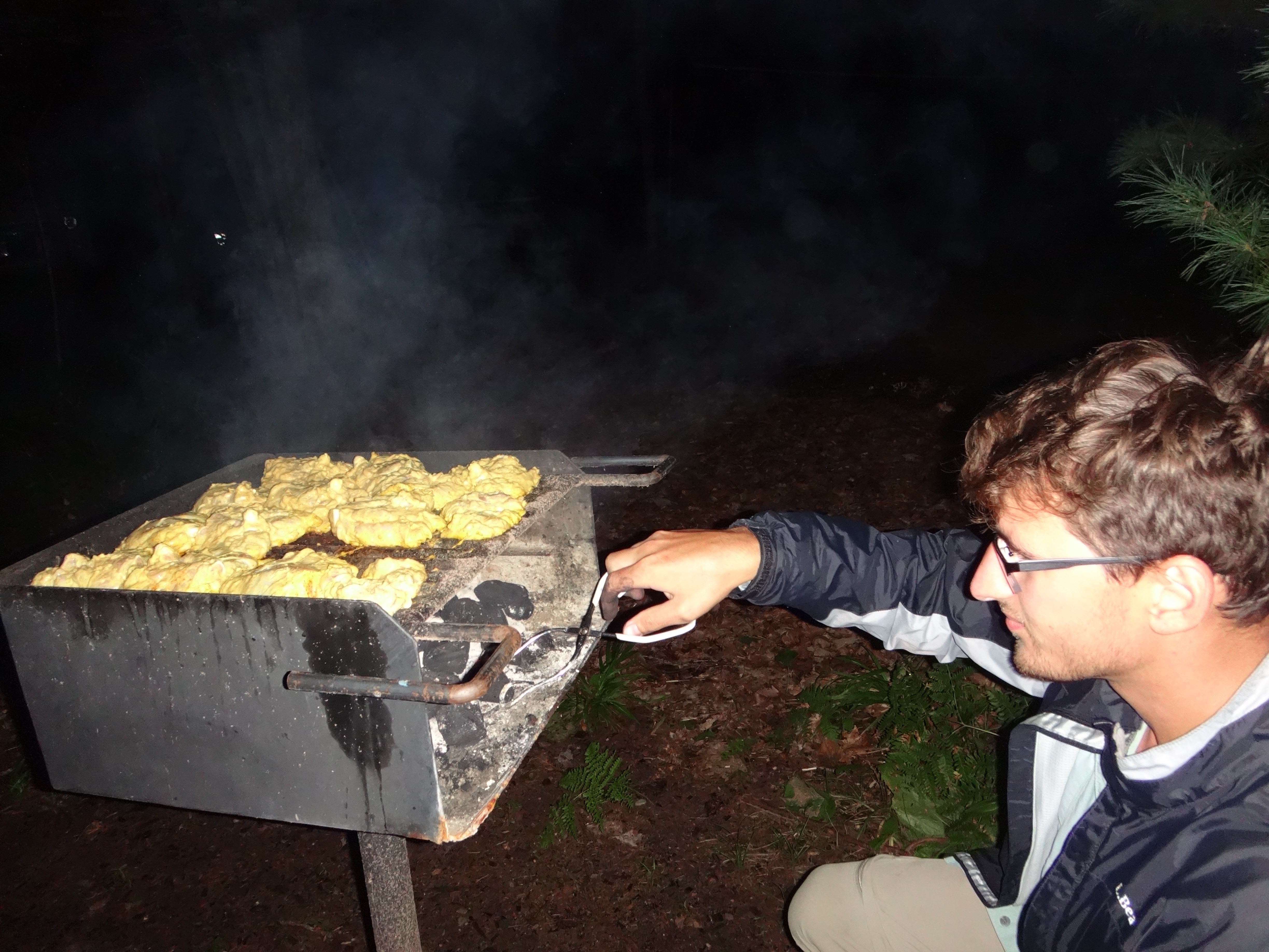
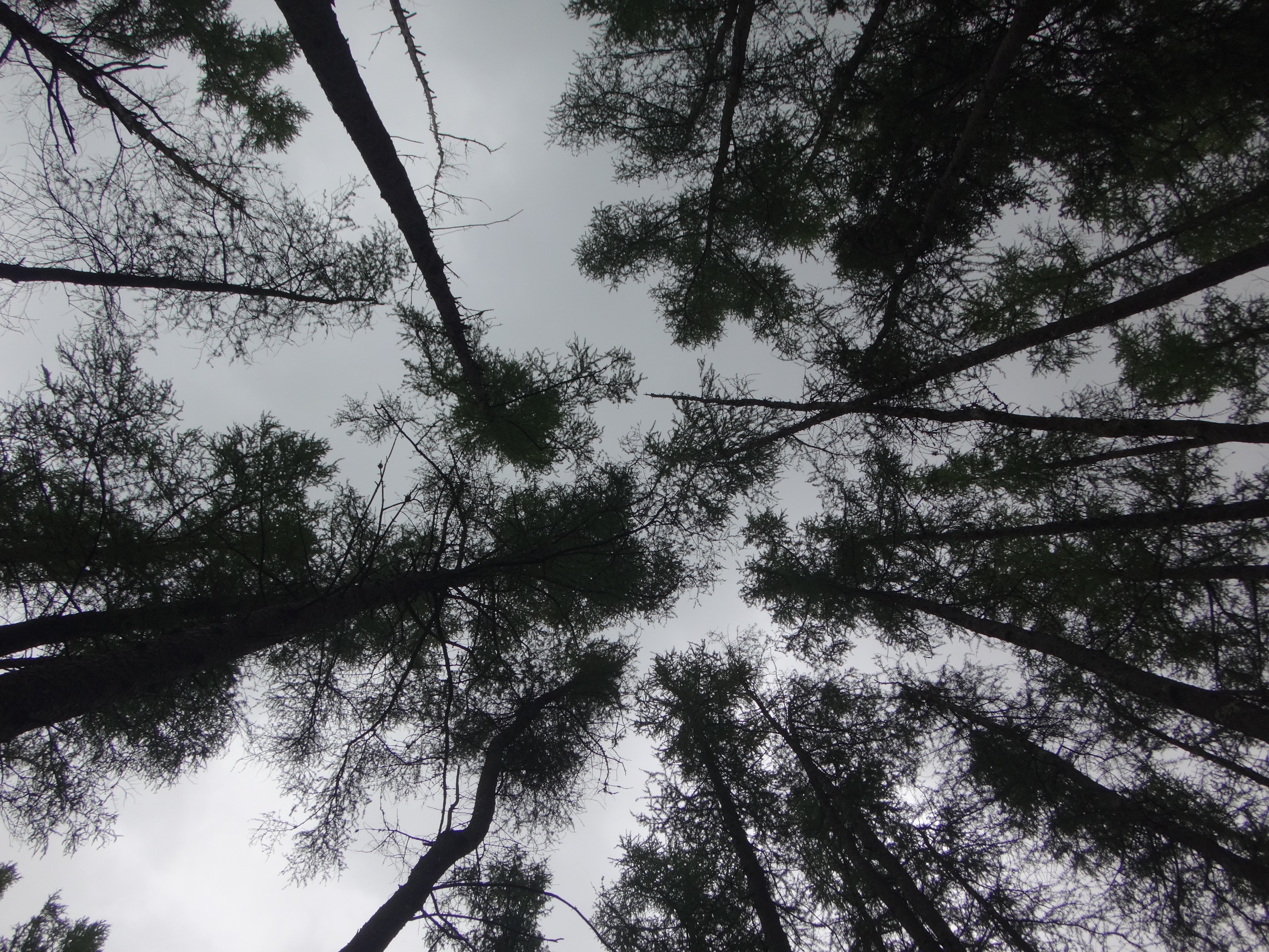
Field work provides the opportunity to be outside, help out on lab-wide projects, and to learn about new research that isn’t exactly in my wheelhouse. September 8-10 I went to the north woods to help collect foliar samples as part of a NEON and Townsend lab project to ultimately predict foliar traits such as morphology, pigments, and other chemical constituents from hyperspectral imagery to create maps of these traits. This was the first year of a five year project. There’s much more to the science behind the goal. But the aim of this post is not to explain all that, but rather, to share some images and the joy of being in the north woods.

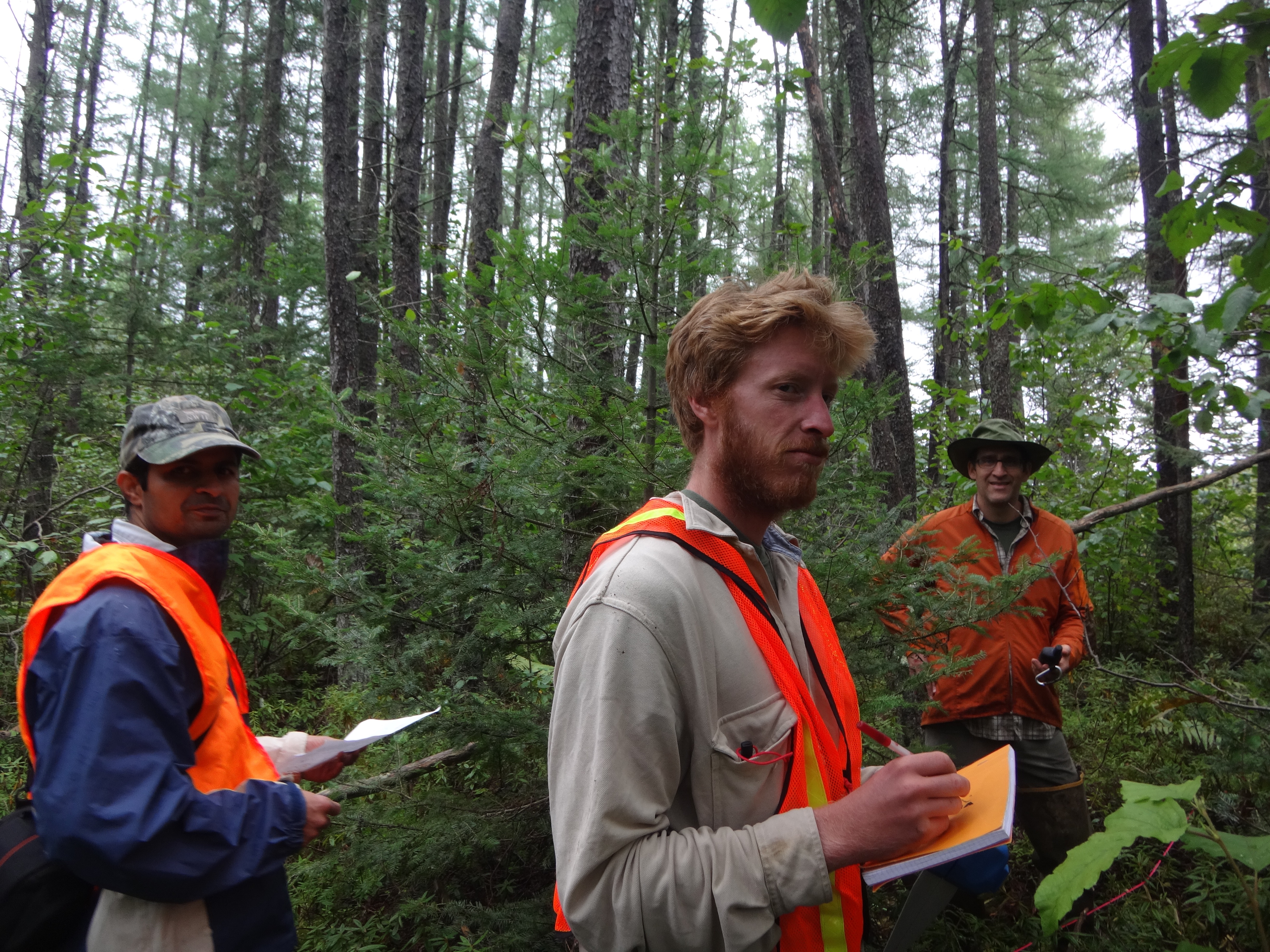
Flux tower of Ankur Desai’s research group, much smaller than NEON’s. Maples creating lovely dappled light.
Making this website orgmode
I use emacs org-mode as the core application for my research. It makes sense to use the great org publishing features to create a website without having to learn many new skills. I had considered using jekyll, but ultimately realized that I could make a website that is just as beautiful and functional with emacs org-mode.
I’ve looked at tons of websites made with org-mode. I like Eric Schulte’s best for an academic personal page, and I wanted to use the org-info.js for a blog with keyboard shortcuts for navigation and search.
If you’re not familiar with org mode, check it out.
If you are already familiar with org mode, spend twenty minutes reading about exporting to html and publishing. The manual is pretty clear. Once you have a published webpage, check out some css stylesheets from other org sites that you like. Mine is a modified version of the stylesheet of eric schulte, who I asked permission from to use.
I spent no more than 3 hours setting up the site. Deciding that this was the approach I wanted to take and generating the content took a couple days.
You can clone the github repo to see how I have it set up.
It is great to be able to work on the content of the website in a very familiar way and export it to the internet with one command. Amazing.
Trip to Washington, DC for NASA’s Biodiversity and Ecological Forecasting Team Meeting nasa travel
Removing Stuck Aluminum Seatpost from a Steel Frame bike life
- In short:
Use a sodium hydroxide solution with proper protection and ventilation. Be patient. Use rubber stoppers to block holes in frame (bottom bracket and water bottle braze-ons.
- In long:
My seatpost had been stuck in my steel frame for years. Fortunately it was at the proper height, so it didn’t bother me. When my headset broke and needed to be replaced, I figured I’d take care of the seatpost at the same time. I wasted an incredible amount of time trying to remove the seatpost and ruined my paint in the process which required a costly repowdering. This post is to share my experience so that you don’t have to go through the same thing.
- What didn’t work:
- Freezing
- Ammonia
- Pipe wrench with 5 foot bar
- combinations of the above
- Tying it between two trees and trying to pull it apart with 3 men and a 6-1 mechanical advantage system.

Figure 70: We pulled hard, but failed - What did work:
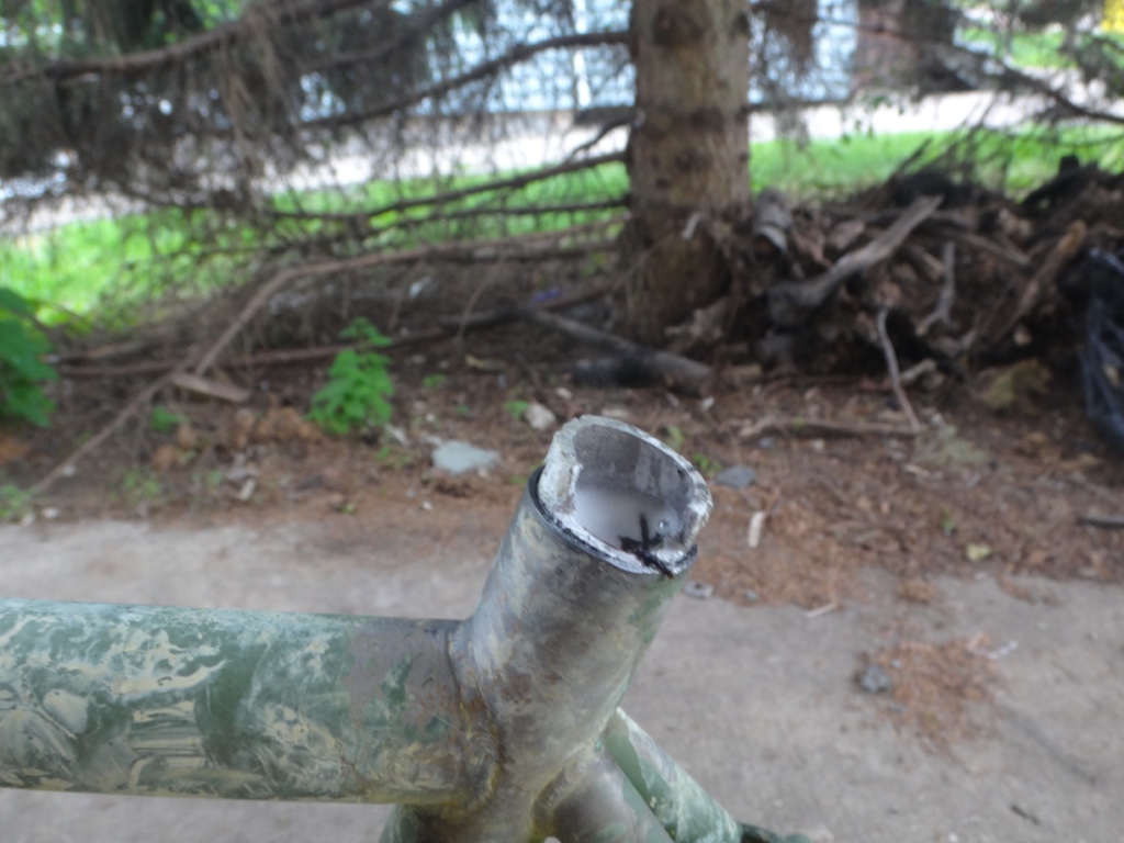
- Remove everything from the frame except the seatpost
- Use a hacksaw to remove seat and create hole to pour solution down. Leave as much of the post as possible to reduce splashing, while still creating a large hole to pour solution down. post in frame, side view
- Stop up bottom bracket and braze-ons (any holes that will let the sodium hydroxide leak out of the seat tube) with rubber or cork stoppers. I got many of different sizes for less than a dollar at the hardware store.
- Place frame in well ventilated area on something to catch any spills (I used a plastic sled in my driveway). setup
- Add sodium hydroxide salt to water (not water to salt). I did this in an old milk jug. Sodium hydroxide is sold at your local hardware store as lye or drain cleaner. Check chemical composition to verify it is NaOH. I didn’t measure the concentration of the solution that I used, but you don’t want it to be so concentrated that it bubbles violently out of seat tube and destroys your paint. Also, the dissolving of NaOH is exothermic and the milk jug will get quite warm, or hot if it’s very concentrated.
- Pour solution into seat tube. The solution needs to be up to the top of the tube so that the part of the post inside the tube will dissolve, but filling it up this high risks spashes. Fill up the tube part way to make sure there isn’t a ton up bubbling and splashing, then fill up to top of tube (not post). If you didn’t saw off too much of the post, this length of post sticking out of tube will help give you a splash buffer. I cut mine too short and the paint was destroyed
- Be patient. My seat post wall was quite thick, at least 2 mm. This will take a long time to dissolve. Wait until the solution is finished reacting with aluminum (you can hear the production of hydrogen gas), which may take a few hours. Then pour out the solution from your frame and dispose of the dark grey liquid (because I wasn’t sure if the NaOH was completely used, I added vinegar in an attempt to neutralize the base).
- Repeat steps 5-7 until the post is completely dissolved or you can pull the post out.
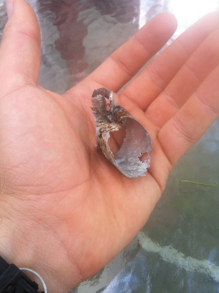
Figure 71: This is all that was left - I had apex custom coating in Monona, WI repaint my frame.
They did a great job and the price was lower than everywhere else I looked, but it still wasn’t cheap. Don’t let the NaOH stay on your frame long!
- What didn’t work:
Fall 2015 hemi video UrbanTrees
references
bibliography:~/git/notes/references.bib