CS 701, Project 2
Global Register Allocation

Due: October 23, 2008 (midnight)
Not accepted after: November 4, 2008 (midnight)

CS 701 focuses primarily on the backend phases of modern compilers. This involves optimization, instruction selection, register allocation and code scheduling.

To reinforce our understanding of the concepts involved, we'll do several projects that implement various backend components. We'll use the LLVM Compiler Infrastructure distributed by the University of Illinois. (LLVM means "Low Level Virtual Machine"). LLVM was developed by a group led by Vikram Adve, an alumnus of the University of Wisconsin. Chris Lattner, Vikram's first Ph.D. student, played a major role in the development of LLVM.

Meet LLVM

LLVM is a compiler framework. Instead of being a single, monolithic program that compiles, assembles, and links a handful of source code files, LLVM supplies multiple programs to handle the various aspects of compilation. Furthermore, the translation from C code to assembly code is broken into several stages: among others, a frontend llvmgcc, an optimizer opt, and a backend llc. LLVM also includes many more tools; most of these are documented at http://llvm.org/docs/CommandGuide/index.html

If we were merely using LLVM as a compiler, this organization would probably be a source of frustration. But since we're working within LLVM, this separation of function gives us many different opportunities to inspect code at various points in the compilation process, helping debugging and keeping the source code simpler.

    source ~cs701-1/public/llvm/scripts/install

    export PATH=$PATH:[INST]/llvm/llvm-2.3/Debug/bin:[INST]/llvm/scripts

    sparc /s/std/bin/cpp foo.c -o foo-pp.c

    llvmgcc -emit-llvm -O0 -c foo-pp.c -o foo.bc

    opt -mem2reg foo.bc -f -o foo.bc

    llvm-dis -f foo.bc

    llvm-as -f foo.ll

    llc -march=sparc -f foo.bc

    sparc /s/std/bin/gcc foo.s -o foo

    sparc foo

int main(int argc, char* argv[]) {
    int n;
    int sum;
    sum = 0;
    for (n = 0; n < 100; n++)
        sum = sum + n*n;
    return sum;
}

; ModuleID = 'bitcode.bc'
target datalayout = "e-p:32:32:32-i1:8:8-i8:8:8-i16:16:16-i32:32:32
-i64:32:64-f32:32:32-f64:32:64-v64:64:64-v128:128:128-a0:0:64-f80:32:32"
target triple = "i386-pc-linux-gnu"

define i32 @main(i32 %argc, i8** %argv) nounwind  {
entry:
        %argc_addr = alloca i32         ; <i32*> [#uses=1]
        %argv_addr = alloca i8**                ; <i8***> [#uses=1]
        %retval = alloca i32            ; <i32*> [#uses=2]
        %sum = alloca i32               ; <i32*> [#uses=4]
        %n = alloca i32         ; <i32*> [#uses=6]
        %tmp = alloca i32               ; <i32*> [#uses=2]
        %"alloca point" = bitcast i32 0 to i32          ; <i32> [#uses=0]
        store i32 %argc, i32* %argc_addr
        store i8** %argv, i8*** %argv_addr
        store i32 0, i32* %sum, align 4
        store i32 0, i32* %n, align 4
        br label %bb8

bb:             ; preds = %bb8
        %tmp1 = load i32* %n, align 4           ; <i32> [#uses=1]
        %tmp2 = load i32* %n, align 4           ; <i32> [#uses=1]
        %tmp3 = mul i32 %tmp1, %tmp2            ; <i32> [#uses=1]
        %tmp4 = load i32* %sum, align 4         ; <i32> [#uses=1]
        %tmp5 = add i32 %tmp3, %tmp4            ; <i32> [#uses=1]
        store i32 %tmp5, i32* %sum, align 4
        %tmp6 = load i32* %n, align 4           ; <i32> [#uses=1]
        %tmp7 = add i32 %tmp6, 1                ; <i32> [#uses=1]
        store i32 %tmp7, i32* %n, align 4
        br label %bb8

bb8:            ; preds = %bb, %entry
        %tmp9 = load i32* %n, align 4           ; <i32> [#uses=1]
        %tmp10 = icmp sle i32 %tmp9, 99         ; <i1> [#uses=1]
        %tmp1011 = zext i1 %tmp10 to i8         ; <i8> [#uses=1]
        %toBool = icmp ne i8 %tmp1011, 0                ; <i1> [#uses=1]
        br i1 %toBool, label %bb, label %bb12

bb12:           ; preds = %bb8
        %tmp13 = load i32* %sum, align 4                ; <i32> [#uses=1]
        store i32 %tmp13, i32* %tmp, align 4
        %tmp14 = load i32* %tmp, align 4                ; <i32> [#uses=1]
        store i32 %tmp14, i32* %retval, align 4
        br label %return

return:         ; preds = %bb12
        %retval15 = load i32* %retval           ; <i32> [#uses=1]
        ret i32 %retval15
}
#include <stdio.h>

• Anything on a line after ; is a comment.
• This file appears to be littered with i32s. As noted here, LLVM is a typed assembly language. i32 denotes a 32-bit integer; i1 denotes a one-bit integer (i.e., a boolean value).
• Virtual registers - that is, assembly-level variable names - each receive an assignment in only one line of the assembly program. That's because the LLVM assembly language is in Single Static Assignment, or SSA form. You'll cover SSA form in greater depth later in 701; for now, understand that every variable is only assigned to by one LLVM instruction, so it is almost trivial to determine the source of a variable's current value.

This LLVM assembly compiles down to the following SPARC assembly:

        .text
        .align  16
        .globl  main
        .type   main, #function
main:
        save -120, %o6, %o6
        st %i0, [%i6+-4]
        st %i1, [%i6+-8]
        sethi 0, %l0
        st %l0, [%i6+-16]
        st %l0, [%i6+-20]
        ba .BB1_2       ! bb8
        nop
.BB1_1: ! bb
        ld [%i6+-20], %l0
        ld [%i6+-16], %l1
        smul %l0, %l0, %l0
        add %l0, %l1, %l0
        st %l0, [%i6+-16]
        ld [%i6+-20], %l0
        add %l0, 1, %l0
        st %l0, [%i6+-20]
.BB1_2: ! bb8
        ld [%i6+-20], %l0
        subcc %l0, 100, %l0
        bl .BB1_1       ! bb
        nop
.BB1_3: ! bb12
        ld [%i6+-16], %l0
        st %l0, [%i6+-24]
        st %l0, [%i6+-12]
.BB1_4: ! return
        ld [%i6+-12], %i0
        restore %g0, %g0, %g0
        retl
        nop

Modifying LLVM

An advantage of LLVM is that even though it's a fully-featured C compiler and is extensible to new languages and other machine targets, its source code is actually fairly sanely engineered. It is not terribly unpleasant to modify LLVM's source code. Another advantage of LLVM is that it has pretty extensive documentation. I recommend that you start with the following pages:

• Read the source code orientation

• Keep handy the LLVM assembly reference

• Skim the page on Bugpoint, an LLVM debugging tool, just so you know that it's available and what it can do.

• Skim Writing an LLVM Pass. You will solve the remaining projects in this class by writing various LLVM passes.

Most of LLVM's function-level documentation is in comments in header files. As such, I've found the source code underlying their Doxygen documentation to be particularly helpful.

Overview of Project 2

To complete Project 2, you'll need to do the following:

• Build a graph class that can print itself in GraphViz format.

• In the Stroll.cpp pass, runnable from opt:

  • Count the number of functions, basic blocks, and instructions in the program, and store these as statistics.
  • Implement the print function of this pass to display the frequency of various kinds of instructions.
  • Use your Graph class to produce a visual CFG of the program's "main" function.

• In RegAllocGraphColoring.cpp, runnable from llc:

  • Do reaching-definitions and live-range analyses.
  • Build live ranges.
  • Display live ranges in the visual CFG.
  • Build a visual interference graph.
  • Perform graph coloring register allocation.
  • Build the visual interference graph, and mark it to show register allocation.
  • Update the IR to use assigned registers; spill unassigned live ranges.

For the grader's sake, while completing Project 2 do not change any files in the LLVM tree except these two. You may add files, but do not change any but Stroll.cpp and RegAllocGraphColoring.cpp.

Draw Pretty Pictures

It will be very useful for you to piece together some sort of Graph class. You'll need this to be able to do live range analysis at an instruction-level granularity. For debugging purposes, it'll be exceedingly useful if your Graph class can print itself in a format that the GraphViz programs dot and neato can read. dot will read a file in this format and draw hierarchical graphs; it's excellent for drawing CFGs. neato reads the same file format, but uses a layout algorithm better tuned to drawing undirected graphs, such as live-range interference graphs.

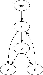
GraphViz syntax is pretty straightforward. A few examples follow, with ugly, un-antialiased images:

digraph { a -> b; b -> c; root -> a; a -> c; b -> d; d -> a; } Compiled with dot:
graph { a [label="First"]; b [label="Second"]; c [label="Most Awesome"] a -- b; b -- c; a -- c; a -- d; d -- e; e -- b; } Compiled with neato:

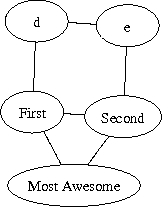
Some of the output formats for dot and neato appear to have some strange issues; however, the scripts dot2pdf and neato2pdf, in the directory llvm/scripts, produce rather handsome pdfs. For instance, the command

    dot2pdf main.dot

will produce main.dot.pdf from the GraphViz file main.dot. GraphViz files can be much more elaborate than these, with labels on edges, colored and shaped nodes, various fonts, and so on. If you're interested in using these more advanced options, you should check out the GraphViz documentation.

Stroll Down the CFG: Stroll.cpp

If you installed LLVM as directed above, you should have an llvm directory that contains a subdirectory llvm-2.3 and a subdirectory scripts. For this part of the project, you'll work on the file:

    llvm/llvm-2.3/lib/Stroll/Stroll.cpp

The class Stroll already here is an opt pass, and its Makefile is configured to build it as a dynamic library. Thus, after we've gotten the Stroll class built and installed, we'll be able to call it from opt as follows:

    llvm/bin/opt -load llvm/lib/Stroll.so -analyze -stroll foo.bc

Exactly what's going on here?

• The -load option loads the compiled Stroll.so as a dynamic library containing opt passes. This convenience allows us to build and test the Stroll pass without needing to repeatedly rebuild the opt binary.
• The -analyze option tells opt that our pass is purely informational; we aren't changing the CFG like an actual optimization pass would, we're just gathering information from it. This also indicates that opt should call Stroll::print() after its execution.
• The -stroll option indicates the pass we'd like opt to run. To see all available passes, try opt -help.
• foo.bc is some bitcode file that we're analyzing.

For more information about opt, see its documentation online.

If you do make && make install from the Stroll directory, and then actually try the above opt command, you'll probably find the output pretty uninformative. Let's make Stroll say a little more about the actual bitcode file it runs upon:

1. One way to get information from a pass driven by opt, llc, or lli is to define statistics, and pass the -stats flag to the driving program. In Stroll.cpp, the FunctionCount statistic is already defined. Given a variable name and a string, the STATISTICS macro defines a global unsigned integer of the given name, and uses the given string as a description of the variable.

   Add statistics to count the total number of basic blocks and instructions in the given module M, and then populate all three statistics with correct values.

2. When opt is called with the -analyze option, it calls the print function of each analysis pass after running that pass's runOn... function. Set up the Stroll pass so that print produces a report giving a count for each of the following disjoint classes of LLVM instructions:

   • Basic-block-terminating instructions
   • Binary operations
   • Memory operations
   • Cast operations
   • PHI nodes
   • All other operations

   The Instruction class has convenient methods to determine an instruction's membership in some of these classes; you'll need to dig a little harder to do others cleanly.

3. The function Function::viewCFGOnly can show you the CFG of a function. Change Stroll so that it displays the CFG of the function main in whatever module it's reading. (The standard method to do this works fine on the CSL machines; if you're doing this project remotely over ssh, you need to configure X forwarding so that it displays nicely.)

   One drawback to using viewCFG or viewCFGOnly is that they're pretty inflexible - you can't change the basic block labels, you can't rewire the graph itself, and you can't get graphs of anything besides basic blocks. So, to make sure that your graph class's output works nicely, and that you're descending the CFG properly, set up the Stroll pass so that it uses your Graph class to print the CFG. Compare this with the output of Function::viewCFG.

Color Graphs: RegAllocGraphColoring.cpp

Build This Code

To actually implement the graph-coloring register allocator, you'll want to edit:

    llvm/llvm-2.3/lib/CodeGen/RegAllocGraphColoring.cpp

While there is a nice, clean way to make opt passes like Stroll.cpp into a dynamic library without needing to recompile and relink the entire system, there is no such convenience for backend components. To do a local build, to at least make sure that your code compiles before linking it all together, you can run make in the CodeGen directory. This will just build object files for changed code.

When you're ready to make a full test build so that you can run your compiler, go to llvm/llvm-2.3 and run make. This can take up to a few minutes. On a multicore machine, you can speed things up a little by passing -jn to make, which instructs it to spawn multiple processes. A good rule of thumb is to set n one larger than the number of processors. Passing -s to make will make it less verbose, which can also yield a noticeable speed boost.

Go ahead and do this build now; RegAllocGraphColoring is initially programmed to spill all registers. So, it is a working register allocator, just a very poorly-performing register allocator. In fact, you should probably go ahead and try running rt on your compiled LLVM compiler.

Now that you're armed with your Graph class, the documentation at http://llvm.org, and the code hooks provided in RegAllocGraphColoring.cpp, you're ready to do live range analysis, and ultimately register allocation.

    DefsOut(b) = {b}

    DefsIn(b0) = {}

    DefsIn(b) = Union (over p in Pred(b)) DefsOut(p)

    DefsOut(b) = DefsIn(b)

   If V is used in b before it is defined in b then
        LiveIn(b) = true
   If V is defined in b before it is used in b then
        LiveIn(b) = false
   If V is neither used nor defined in b then
        LiveIn(b) = LiveOut(b)

    LiveOut(b) = OR (over s in Succ(b)) LiveIn(s)

   Range(b) = b Union {k | b in DefsIn(k) AND LiveIn(k)}

   If Range1 Intersect Range2 is non-empty
   Then union together Range1 and Range2 into one composite live range

1. Assume we have R registers (colors). Any node that has fewer than R neighbors can always be colored. Remove it from the interference graph and push it on a stack.

2. Repeat step (1) until the graph is empty or no more nodes can be removed. If the graph is empty do step (4).

3. For each remaining node compute the cost of not assigning it a register. This cost is number of extra instructions needed if the live range must load and store values from memory. Scale each added instruction by a factor of 10**nest, where nest is the loop nesting level at which the instruction appears.

   Let n be the number of neighbors a node has. Select that node which has the smallest value of cost/n. Remove it from the graph and push it on a stack. Return to step (1).

4. Pop each node from the stack. If its neighbors use fewer than R colors, give it any color that doesn't interfere. Otherwise, discard the node.

When you've decided which live ranges are to be allocated a particular register you will then direct the code generator to directly reference that register rather than use the virtual register.

Allocate Registers: RegAllocGraphColoring.cpp

First, you should look at the documentation for the LLVM target-independent register allocator

In particular, understand that LLVM actually provides an layer of abstraction between details of a machine's architecture and a register allocator; in the code, these are mostly in classes that begin with Target. Thus, you want to isolate decisions about the target architecture to those. If you do so correctly, your register allocator will work on any architecture for which LLVM has a backend. However, your register allocator will only be graded for its performance on SPARC machines.

Things that get called "registers" in LLVM can be either "physical" or "virtual" registers. Really, a register is just an unsigned integer, used as a token to manage the resource, rather like a Unix file handle. Except for instructions which are defined to target specific physical registers (arithmetic error flags, for instance, or the arithmetic accumulator in X86), the program entering register allocation uses entirely virtual registers. After register allocation, it must contain only physical registers. Physical and virtual registers use the same numberspace: a register is a physical register if it's between 0 and the number of registers in the architecture, and it's otherwise a virtual register. For safety's sake, though, you should do such checks in your code via TargetRegisterInfo::isVirtualRegister().

You are not required to allocate floating-point registers. (You can do so for extra credit, but you will have to handle register aliases (single vs. double length registers) and saving and restoring registers around subprogram calls.) You can tell if a register is floating-point by the TargetRegisterClass to which it belongs. In particular, on the SPARC, TargetRegisterInfo::getRegClass(n) yields floating point TargetRegisterClass for n equal to 1 and 2, and yields the integer/pointer TargetRegisterClass for n equal to 3.

Important Classes

MachineFunction: The top-level data class that gets handed to your register allocator. It leads to details about both the target machine and the LLVM code of the current function.

TargetMachine: Contains mostly accessor functions to data classes. The objects returned by TargetMachine::get*() functions generally hold the answers to queries about the target architecture.

MachineInstruction: You could need almost any method of this class. This matters.

MachineOperand: This class's header has several sections; you may need the parts that regard register operands.

Key Functions

This is by no means a complete list, but it contains a few important functions that you're bound to call. These are explained pretty fully in their headers.

• TargetMachine::getRegClass(virtual_register)
• TargetMachine::setPhysReqUsed(physical_register)
• TargetMachine::setPhysReqUnused(physical_register)
• TargetRegisterInfo::isVirtualRegister(register)
• MachineInstruction::getOperand(i)
• MachineOperand::setReg(physical_register)

The TargetInstrInfo class contains quite a few methods for inserting instruction that you'll need, like storing and loading registers to or from stack locations. In particular, you may need: - TargetInstrInfo::copyRegToReg - TargetInstrInfo::storeRegToStackSlot - TargetInstrInfo::loadRegFromStackSlot

The Backup Allocator

If you've looked at RegAllocGraphColoring.cpp already, you've probably noticed that its callback function instantiates the class RegAllocBackup and calls its allocate_regs() method. RegAllocBackup is a simple, stupid register allocator, set up specifically to run on the SPARC. Calling its allocate_regs() method will perform semantically-correct but extremely inefficient register allocation on all virtual registers that remain in the MachineFunction with which it was initialized. This is initially in the runOnMachineFunction method of RegAllocGraphColoring; leave it there to let it handle floating-point registers and cases that you may have missed.

RegAllocBackup needs to keep a handful of registers to itself, to use as temporary storage. In any event, you'll want your allocator to allocate no more than 16 registers, the locals and in registers (global and out registers aren't protected across subprogram calls). In initial testing may want to allocate even fewer registers (perhaps only one or two local registers). This will allow you to test correct operation on small test programs that need (at most) only a few registers. For any TargetRegisterClass *rc, the value of RegAllocBackup::numUsableRegs(rc) returns the number of registers that your allocator can work with. So, if you use only registers obtained by rc->getRegister(i) for
0 <= i < RegAllocBackup::numUsableRegs(rc), then your register allocator and RegAllocBackup will not interfere. In any case, RegAllocBackup::numUsableRegs(rc) controls the number of registers you choose to allocate and TargetRegisterInfo::getRegister(n) determines which physical register is actually allocated.

If your final register allocator works without this safety net - you don't call RegAllocBackup, and you allocate floating-point registers yourself - then you will earn extra credit.

Check Your Work

    count-inst myprog

will instrument the SPARC executable myprog, run the instrumented program on a SPARC machine, and print the number of instructions executed in the instrumented run. If you want more detailed profiling information, feel free to copy and edit count-inst, and consult the QPT manpages: qpt2, qpt2_stats.

If the file myprog.input exists in the same directory as myprog, the count-inst will pipe the input file into myprog's standard input when it runs and measures myprog. If myprog.input does not exist there, count-inst will assume that the program doesn't expect to read from standard input.

You should use QPT to ensure that your optimized code outperforms code without those optimizations; more detailed reports can tell you exactly how many loads and stores the compiled code executes.

Submit Your Work

This project may be done individually or in two person teams. Grading requirements will be relaxed for one person implementations, especially for flawed or incomplete implementations. Assignments handed in late will be penalized 3% per day, up to a maximum of 21% for assignments handed in on October 30th.

Copy the following to your subdirectory in ~cs701-1/public/proj2/handin:

• Stroll.cpp
• RegAllocGraphColoring.cpp
• Any files that are necessary to compile your Stroll.cpp and RegAllocGraphColoring.cpp that weren't in the original LLVM tree. (For instance, your graph class, if that's in a separate file.)
• A file named README that tells where your new files should be placed before building. In the case that you did work for extra credit, note what work was done and where it can be found in your code. For instance, if you added a header named GraphPrinter.h to the main include directory, mention the file like llvm/llvm-2.3/include/GraphPrinter.h in your README file.

Good Luck! (And start early -- 3 weeks can pass rather quickly).