
1.   k = 2;
2.   if (...) {
3.      a = k + 2;
4.      x = 5;
5.   } else {
6.      a = k * 2;
7.      x = 8;
8.   }
9.   k = a;
10.  while (...) {
11.     b = 2;
12.     x = a + k;
13.     y = a * b;
14.     k++;
15.  }
16.  print(a+x);
Constant Propagation
The goal of constant propagation is to determine where in the program variables are guaranteed to have constant values. More specifically, the information computed for each CFG node n is a mapping from variables to values (where a variable x is mapped to a value v at node n if x is guaranteed to have value v whenever n is reached during program execution). Below is the CFG for the example program, annotated with constant-propagation information.
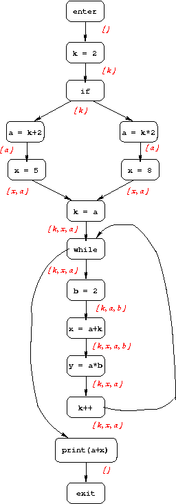
Live-Variable Analysis
The goal of live-variable analysis is to determine which variables are "live" at each point in the program; a variable is live if its current value might be used before being overwritten. The information computed for each CFG node is the set of variables that are live immediately after that node. Below is the CFG for the example program, annotated with live variable information.
Draw the CFG for the following program, and annotate it with constant-propagation and live-variable information.
N = 10;
k = 1;
prod = 1;
MAX = 9999;
while (k <= N) {
  read(num);
  if (MAX/num < prod) {
      print("cannot compute prod");
      break;
  }
  prod = prod * num;
  k++;
}
print(prod);
Return to Dataflow Analysis table of contents.
Go to the previous section.
Go to the next section.