CS368 Homework 4
Lec 2, Spring 2016
Due by 11:59 pm on Friday, March 18 (not accepted late)
Announcements
Check here periodically.
| 3/8/2016 | Homework assigned. To ask questions about the homework and see questions posed by other students and their answers, go to: http://www.piazza.com/wisc/spring2016/cs368 and sign-in using your wisc.edu account. |
Problems
Please note: Your solution must use techniques that have been discussed and covered in lecture and the on-line readings. Your solution may not use MATLAB commands or constructs that have not been covered in lecture prior to the date of the release of the homework (or in the corresponding on-line readings).
For this homework create one main script file named homework4.m and the supporting function named heatPlate (in a file named heatPlate.m). Define the function as it is specified and then, in the main script file, correctly call the function to solve the problem. You can download this MATLAB script to get started: homework4.m
Problem 1: (7 points) Interpolation
Computer-controlled machines are used to cut and to form metal and other materials when manufacturing products. These machines often use interpolating functions (such as splines) to specify the path to be cut or the contour of the part to be shaped. The data in this table represents the shape of a car's front fender (units are in feet).
| x data | 0 | 0.25 | 0.75 | 1.25 |
1.5 | 1.75 | 1.875 | 2 |
2.125 |
2.25 |
|---|---|---|---|---|---|---|---|---|---|---|
| y data | 1.2 |
1.18 |
1.1 |
1 |
0.92 |
0.8 |
0.7 |
0.55 |
0.35 |
0 |
-
Interpolate the data using a polynomial that goes through all the data points. (Make sure to display the coefficients you get for the interpolating polynomial.)
-
Plot the data points and the interpolating polynomial through all the data points over the range x = 0 to 2.25 on a single figure. Use green diamonds to represent the data points and a black dash-dot line for the polynomial. Use the axis command to scale the plot so that x ranges from 0 to 2.25 and y ranges from 0 to 1.5.
-
Plot the spline interpolation through the same data points on the same figure as part b. Use a red solid line for the spline.
-
For x = 0.5, find the corresponding estimated y values using your polynomial interpolation and your spline interpolation. Use a disp command to display your results along with text that makes it clear which technique was used to produce each estimate.
Problem 2: (6 points) Approximation
For the data in the following table, the y data obviously decays as x increases:
| x data | 1.00 | 2.12 | 3.09 | 5.23 |
7.64 | 9.14 | 11.2 | 14.3 |
16.1 | 18.3 | 22.7 |
25.0 |
|---|---|---|---|---|---|---|---|---|---|---|---|---|
| y data | 2.43 |
2.21 |
2.07 |
1.79 |
1.63 |
1.58 |
1.49 |
1.42 |
1.39 |
1.34 |
1.27 |
1.24 |
Fit this data to a curve of the form:
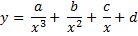
(Hint: transform the curve to a polynomial in y and u = 1/x)
Make sure to display the values for a, b, c, and d.
-
Plot the data points and approximating function over the range x = 1 to 25 on a single figure. Use diamonds to represent the data points and a red dash-dot line for the approximating curve.
Estimate the value of y at x = 10.5 using your approximating function.
Problem 3: (7 points) Heat Plate
We can determine the temperature at various locations across a heat plate by modeling such a problem as a system of linear equations and solving the linear system in MATLAB.
Imagine that you wish to know the temperature at all points on a plate that is insulated except for two positions on the edge where heating elements of known temperature are applied. At some point when the temperature at all positions on the plate have stabilized, what will the temperature at each point be?
To solve such a problem, we imagine the plate surface divided into equal sized "tiles" and restate the problem to find the temperature at the center of each tile. We know that the temperature of each tile depends upon its neighboring temperatures. In fact, it is a weighted average of those temperatures based on the proportion of our tile's edge that is shared with its neighbor. Here is a square "plate" divided into 9 equal area tiles. Assume that each edge of each tile has identical length, so that the temperature of any one tile is a simple average of the temperatures of all neighboring tiles that share a side with the tile in question. This creates a system of 9 equations, one for each "tile" area.
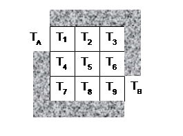
TA and TB are the non-insulated positions along the edge where a heat source of known temperature will be applied. The temperatures at T1 through T9 are the unknowns that you wish to find.
To solve this problem, identify 9 equations. Each equation represents the temperature value for one tile based upon the temperature values of each of its neighboring tiles. For example, the temperature at T5 is equal to the average of the temperatures: T2, T4, T6, and T8.
What about the corners? Well, since the gray area is insulation, the only effect is from the non-insulating tiles. Thus, T3 is equal to the average of only T2 and T6.
How do TA and TB factor into the equations? They will be in the equations, but since their values will be known when the function is called, the terms with TA and TB should be on the right-hand side of the equations once the equations are reordered.
DO NOT SOLVE FOR ANY OF THE TEMPERATURES OF THIS PROBLEM BY HAND. Work out the equations for each tile and then reorder the terms in general form, with the unknown terms on the left-hand side and the known terms on the right-hand side of the equation. Once you have the equations, rewrite the linear system as a matrix equation and put the commands to solve this problem in your heatPlate(TA,TB) function definition.
-
In a comment in your homework4 script, give the nine equations for this linear system, one linear equation for each unknown temperature, T1 through T9.
-
Define a function named heatPlate that accepts two temperature values TA and TB (representing TA and TB, respectively) and returns a single matrix result that is a 3x3 matrix of temperatures for the unknowns T1 through T9 in the order labeled above. If you can not figure out how to return the values as a 3x3 matrix, return them as a column vector for a minor (1/2 pt) deduction.
Hint: first rewrite your system of equations from part a as a matrix equation, with a coefficient matrix, vector of unknowns, and a data vector (right-hand side of the equation).
-
In your homework4 script, write code to call your heatPlate function to compute the values of T1 through T9 when TA = 50 and TB = 75 and display the results.
Handing in
Upload your m-files to your Dropbox in Learn@UW. See these instructions for uploading files to a Learn@UW Dropbox. The files you should upload are:
- homework4.m
- heatPlate.m
In order for your work to be considered to have been turned in on-time, you must upload your files to your Learn@UW Dropbox by 11:59 pm Friday, March 18.