CS766 Computer Vision, Fall 2007
Project 3: Photometric Stereo
Assigned: Oct 10, 2007
Due: Oct 24 noon, 2007
The instructor is extremely thankful to Prof Steve Seitz for allowing us to use this project which was developed in his Computer Vision class.
Project Description
In this project, you will implement a system to construct a height field from a series of images of a diffuse object under different point light sources. Your software will be able to calibrate the lighting directions, find the best fit normal and albedo at each pixel, then find a surface which best matches the solved normals. Unlike the previous two projects, we provide all experimental images and you are not required to take photos. However, you are welcome to check out cameras and acquire your own images for extra credits. We highly recommend you to do this project in Matlab. If you are not familiar with it, here is a jump start.
Here are the steps.
1. Calibration. Before we can extract normals from images, we have to calibrate our capture setup. This includes determining the lighting intensity and direction, as well as the camera response function. For this project, we have already taken care of two of these tasks: First, we have linearized the camera response function, so you can treat pixel values as intensities. Second, we have balanced all the light sources to each other, so that they all appear to have the same brightness. You'll be solving for albedos relative to this brightness, which you can just assume is 1 in some arbitrary units. In other words, you don't need to think too much about the intensity of the light sources.
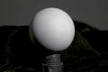
The one remaining calibration step we have left for you is calibrating lighting directions. One method of determining the direction of point light sources is to photograph a shiny chrome sphere in the same location as all the other objects. Since we know the shape of this object, we can determine the normal at any given point on its surface, and therefore we can also compute the reflection direction for the brightest spot on the surface.
2. Normals from Images.
The appearance of diffuse objects can be modeled as ![]() where I is the pixel intensity, kd is the albedo, and L is the lighting direction (a unit vector), and n is the unit surface normal. (Since our images are already balanced as described above, we can assume the incoming radiance from each light is 1.) Assuming a single color channel, we can rewrite this as
where I is the pixel intensity, kd is the albedo, and L is the lighting direction (a unit vector), and n is the unit surface normal. (Since our images are already balanced as described above, we can assume the incoming radiance from each light is 1.) Assuming a single color channel, we can rewrite this as ![]() so the unknowns are together. With three or more different image samples under different lighting, we can solve for the product
so the unknowns are together. With three or more different image samples under different lighting, we can solve for the product ![]() by solving a linear least squares problem. The objective function is:
by solving a linear least squares problem. The objective function is:
![]()
To help deal with shadows and noise in dark pixels, its helpful to weight the solution by the pixel intensity: in other words, multiply by Ii:
![]()
The objective Q is then minimized with respect to g. Once we have the vector g = kd * n, the length of the vector is kd and the normalized direction gives n.
Weighting each term by the image intensity reduces the influence of shadowed regions; however, it has the drawback of overweighting saturated pixels, due to specular highlights, for example. You can use the same weighting scheme we used in the project 1 to address this issue.
3. Solving for color albedo.
This gives a way to get the normal and albedo for one color channel. Once we have a normal n for each pixel, we can solve for the albedos by another least squares solution. But this one ends up being a simple projection. The objective function is
![]()
To minimize it, differentiate with respect to kd, and set to zero:
![]()
![]()
Writing Ji = Li . n, we can also write this more concisely as a ratio of dot products: ![]() This can be done for each channel independently to obtain a per-channel albedo.
This can be done for each channel independently to obtain a per-channel albedo.
4. Least square surface fitting. Next we'll have to find a surface which has these normals. We will again use a least-squares technique to find the surface that best fits these normals. Here's one way of posing this problem as a least squares optimization:
If the normals are perpendicular to the surface, then they'll be perpendicular to any vector on the surface. We can construct vectors on the surface using the edges that will be formed by neighbouring pixels in the height map. Consider a pixel (i,j) and its neighbour to the right. They will have an edge with direction
(i+1, j, z(i+1,j)) - (i, j, z(i,j)) = (1, 0, z(i+1,j) - z(i,j))
This vector is perpendicular to the normal n, which means its dot product with n will be zero:
(1, 0, z(i+1,j) - z(i,j)) . n = 0
![]()
Similarly, in the vertical direction:
![]()
We can construct similar constraints for all of the pixels which have neighbours, which gives us roughly twice as many constraints as unknowns (the z values). These can be written as the matrix equation Mz = v. The least squares solution solves the equation ![]() However, the matrix
However, the matrix ![]() will still be really really big! It will have as many rows and columns as their are pixels in your image. Even for a small image of 100x100 pixels, the matrix will have 10^8 entries!
will still be really really big! It will have as many rows and columns as their are pixels in your image. Even for a small image of 100x100 pixels, the matrix will have 10^8 entries!
We suggest two ways for you to try out. (a) most of the entries are zero, and there are some clever ways of representing such matrices and in Matlab, called sparse matrices. You can figure out where those non-zero values are, put them in a sparse matrix, and then solve the linear system. (b) there are iterative algorithms that allow you to solve linear system without explictly storing the matrix in memory, such as the conjugate gradient method. The main task for you is to write a matlab function that multiplies ![]() and z. Pleaes read Mablat help for more details. You can also find out more details about the Conjugate Gradient method here.
and z. Pleaes read Mablat help for more details. You can also find out more details about the Conjugate Gradient method here.
After computing the surface, you can use Matlab to plot it. surfl works best for this project.
Experiment Data
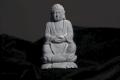
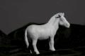
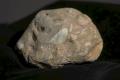
We have provided six different datasets of diffuse (or nearly diffuse) objects for you to try out:
|
|
|
|
|
|
gray |
buddha |
horse |
cat |
owl |
rock |
They can be downloaded here here.
After you unzip it, you will see seven directories. They correspond to the above six objects and a chrome ball. Each of the directory has 11 images under different lightings. The chrome ball images can be used to compute lighting directions for computing normal maps for other six objects.
Under each of the directory, there is also a mask image. Thoses indicates what pixels are on the objects. You only need to estimate normals and compute height values for these.
From the chrome ball images, you should estimate the lighting directions. Here are some hints:
Bonus Points
Here is a list of suggestions for extending the program for extra credit. You are encouraged to come up with your own extensions. We're always interested in seeing new, unanticipated approaches and results!
You are welcome to do any other extensions or develop algorithm related to image mosaics. The bonus depends on how useful and difficult these extensions are.
Submission