Figure 1: selected image showing successful calibration.
The red line points in the direction of the lighting direction vector.
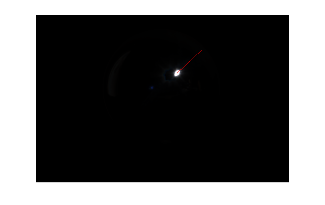
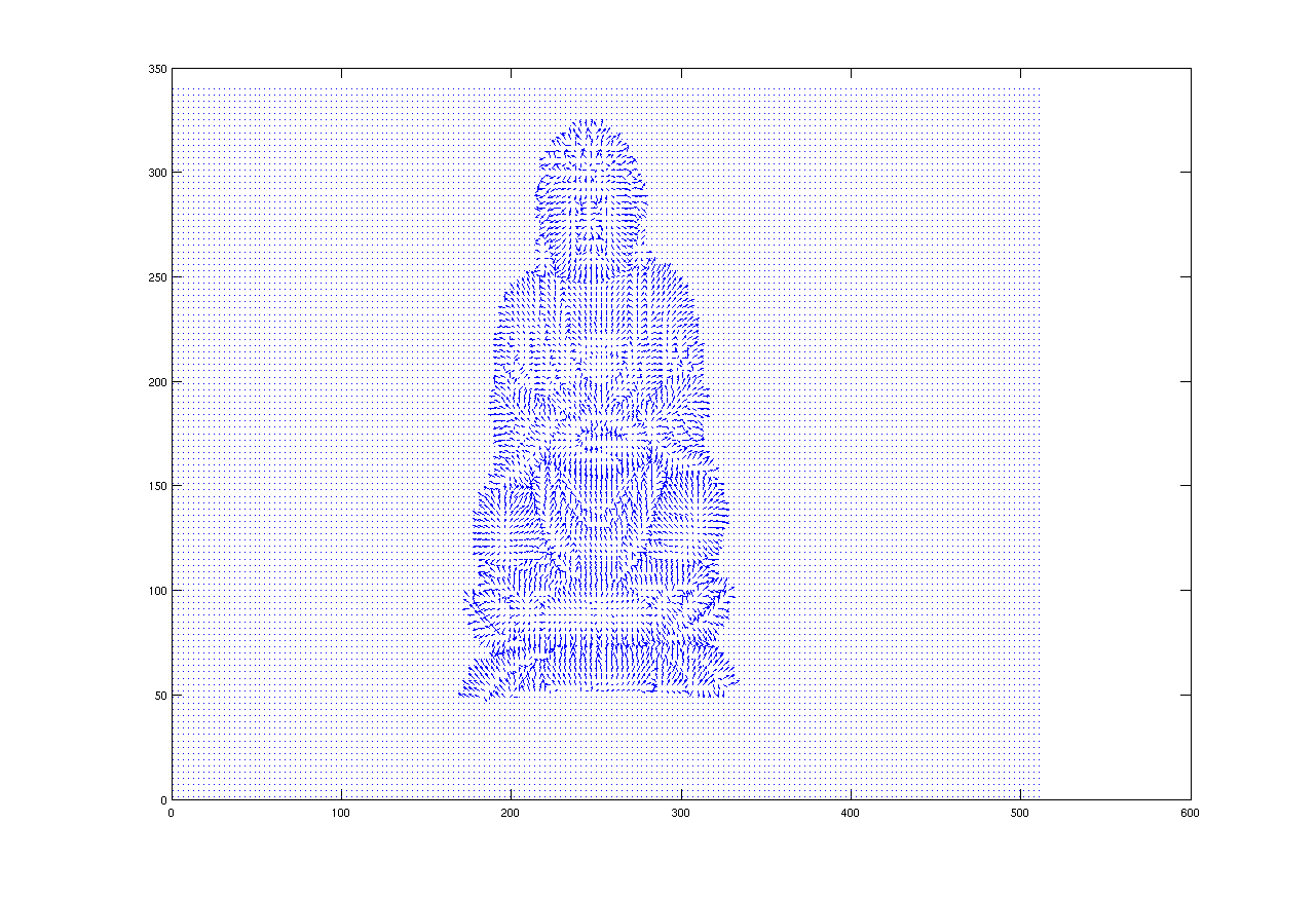
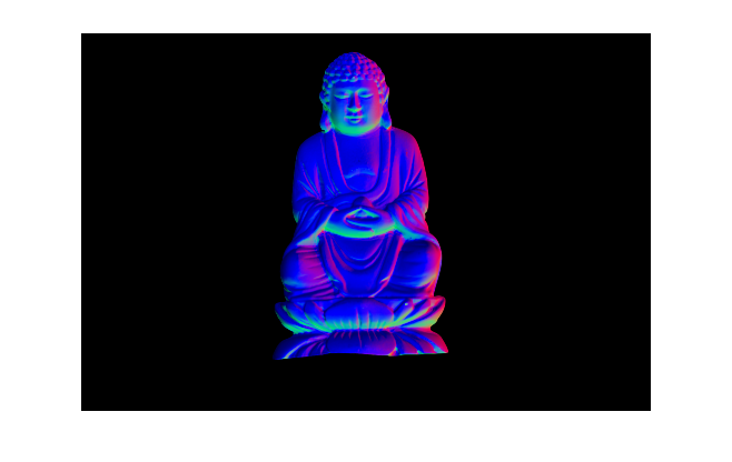
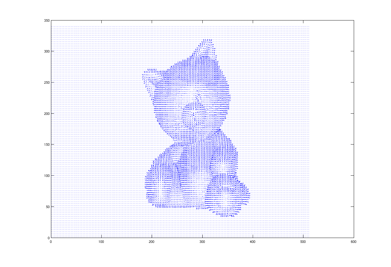
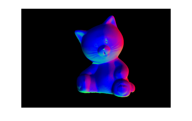
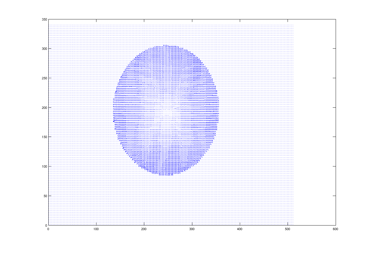
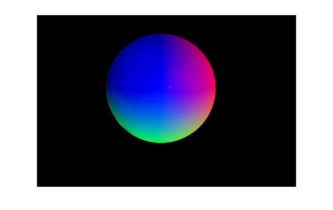
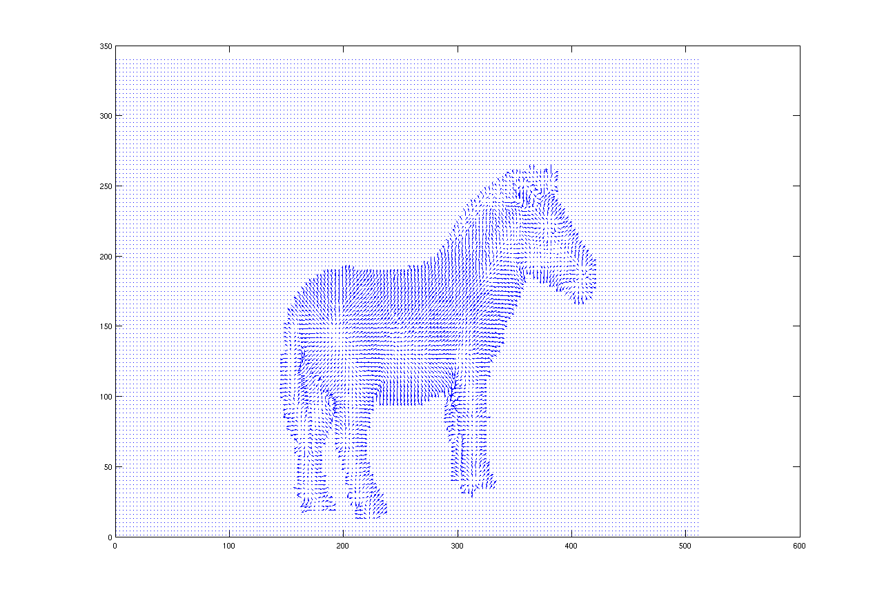
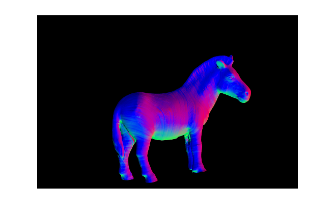
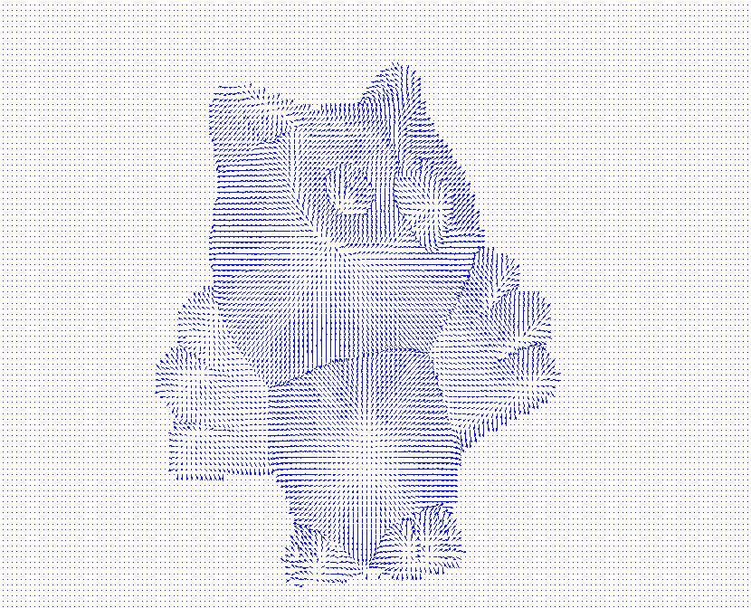
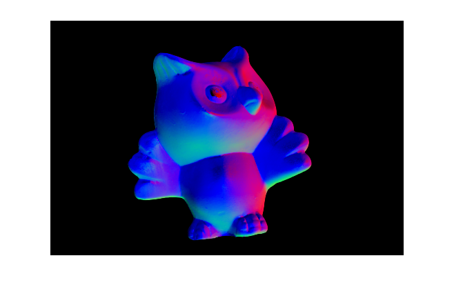
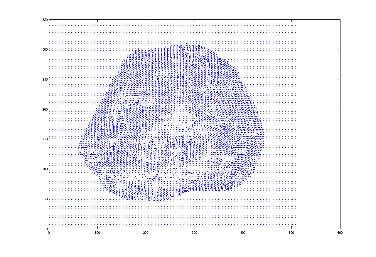
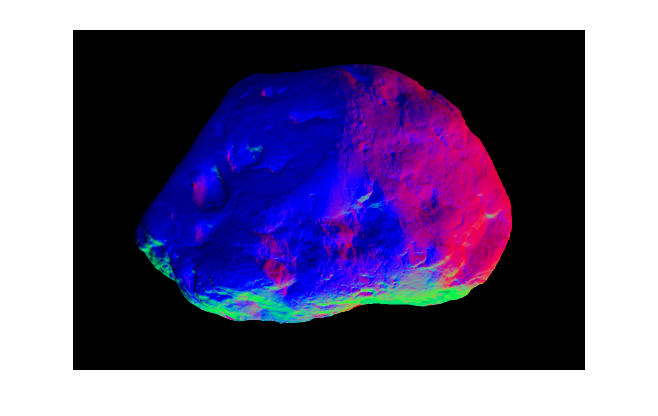
Figure 2: surface normal vectors shown using arrows and by RGB-encoding
Brandon M. Smith
Outline
Introduction
Approach
Results
List of Submitted Files
References
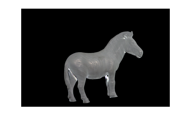
The objective of this project was to create a 3D image based on a series of 2D images using a technique called photometric stereo. Each set of 2D images depicts the same object in the same location. The only difference between the images in each set is that the light used to illuminate the object is moved. If we know the lighting direction for each image, we can obtain the surface normal vectors on the surface of the object. Then, using a system of equations, we can use these surface normal vectors to find a good approximation of the 3D surface of the object.
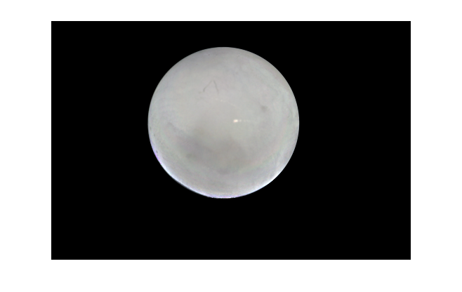
In order to determine the lighting direction for each image, we first calibrate the capture setup. This is done using a set of images of a chrome sphere. We can determine the lighting direction for each image based on the location of a bright spot on the sphere. Figure 1 shows this.
All of the “code” for this project was written in MATLAB. To use the program, simply move to the program directory and type the following in MATLAB:
photometricStereo('../psmImages/chrome.txt', '../psmImages/cat.txt');
where the first string is the name of the file containing the names of the chrome images used to calibrate the capture setup, and the second string is the name of the file containing the names of the images used to generate the results. Everything is taken care of from here. The images required for the project (i.e., albedo map, 3D image, etc.) are automatically displaying in separate figures.
The first step was to calibration the capture setup. To verify that a) my program was finding the center of the bright spot accurately, and b) determining the lighting direction vector properly, I generated some images with the lighting direction vector superimposed on the corresponding calibration image. This is shown in Figure 1.
The next step was determining the surface normal vectors for each object. We can get a sense of the normal vectors in 2D by looking at an image composed of small arrows (i.e., using MATLABs quiver command), or by encoding them in red-, green-, and blue-channels of an image. The surface normals for each object in both representations are shown in Figure 2.
Figure 1: selected image showing successful calibration.
The red line points in the direction of the lighting direction vector.
Figure 2: surface normal vectors shown using arrows and by RGB-encoding
 |
 |
 |
 |
 |
 |
 |
 |
 |
 |
 |
 |
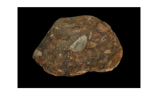
The albedos for each object were also obtained and are shown in Figure 3.
Figure 3: (color) albedos for each object
 |
 |
 |
 |
 |
 |
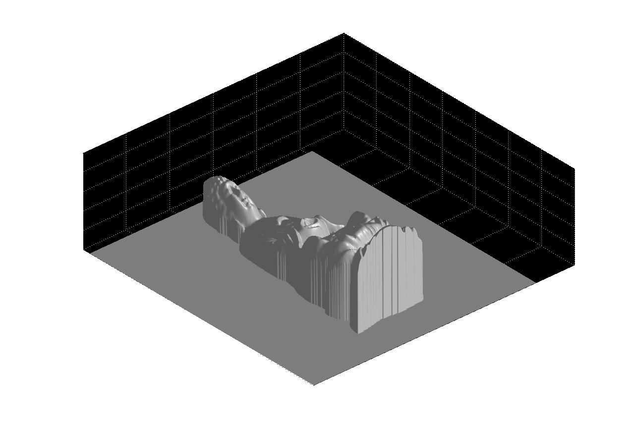
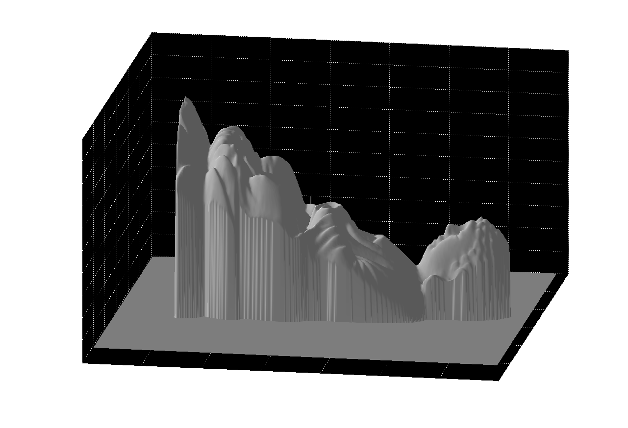
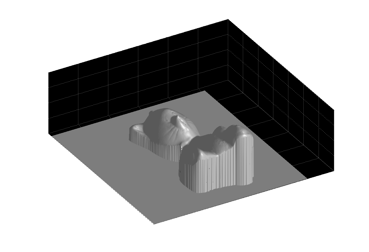
The final step was to assemble a (large!) system of equations with surface depths
as the unknowns and the normal vector components as the knowns. The z-components
of the normal vectors were arranged into a large sparse matrix A, and the x-
and y- components of the normal vectors were assembled into a column vector
b. This produced an over-constrained system in the form
Az = b,
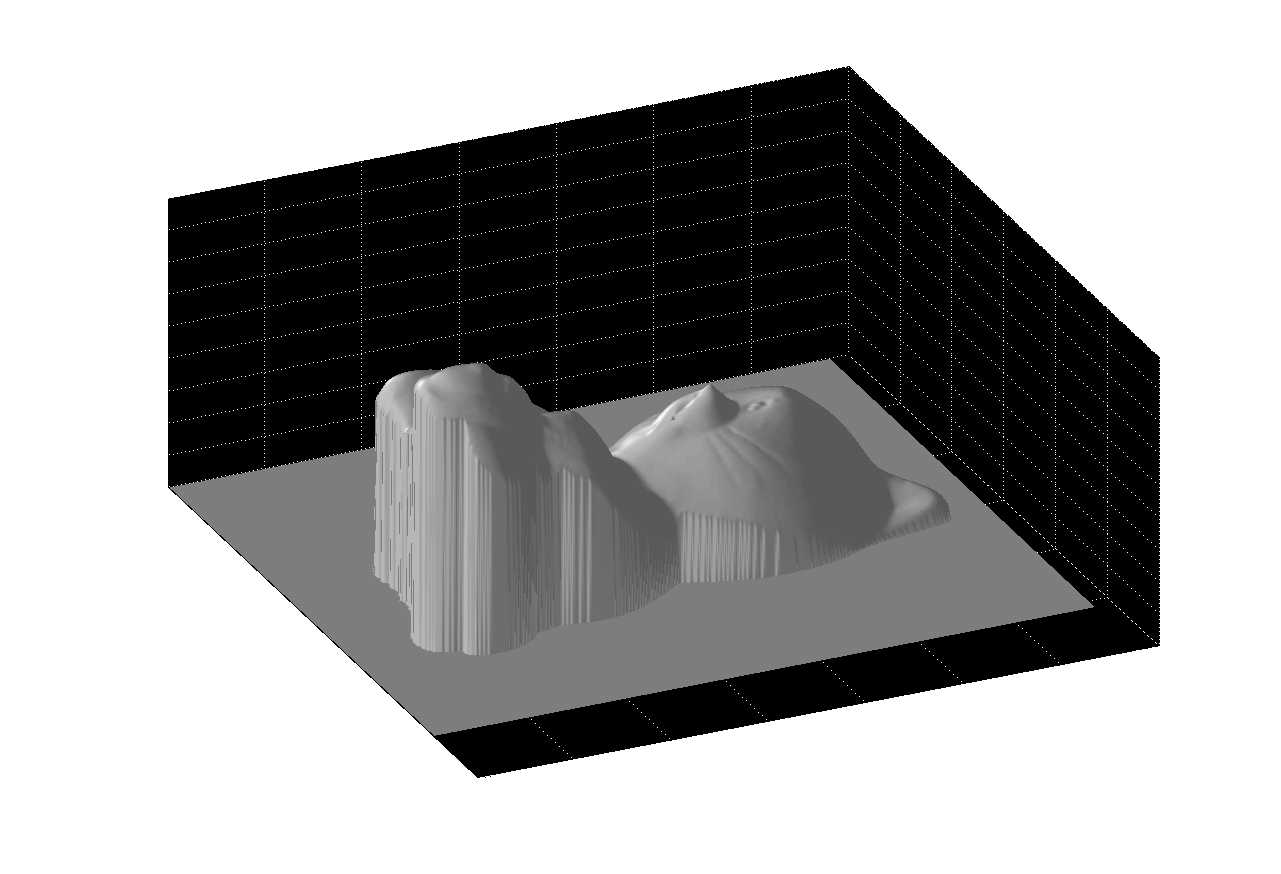
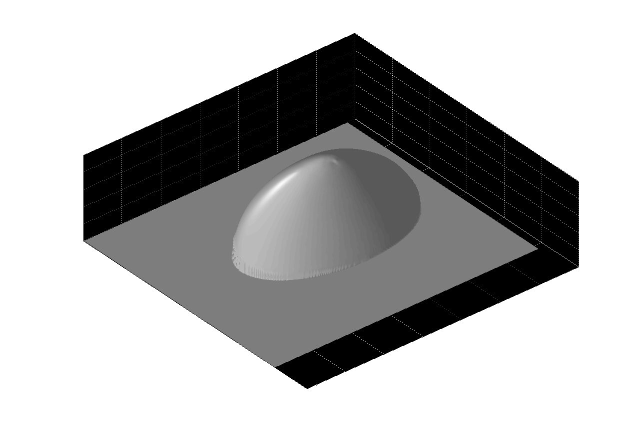
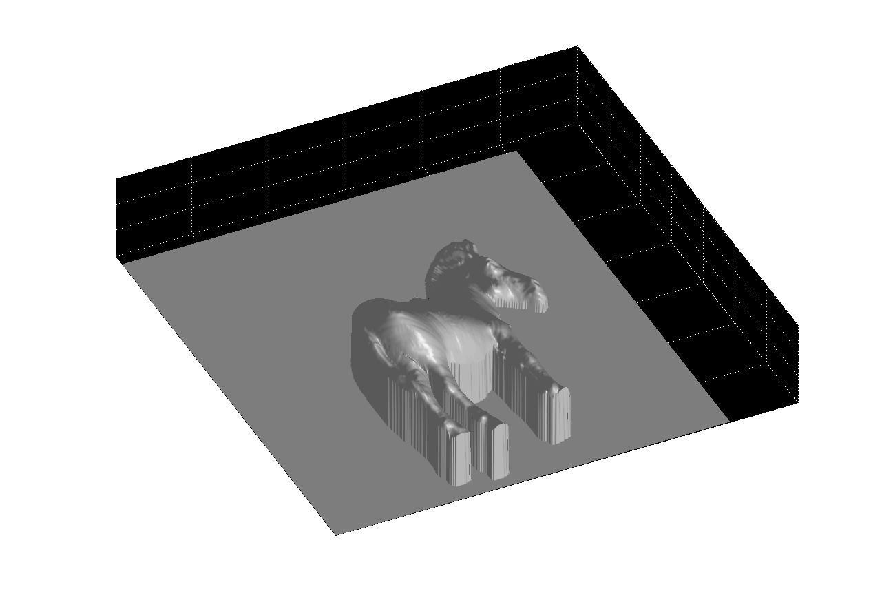
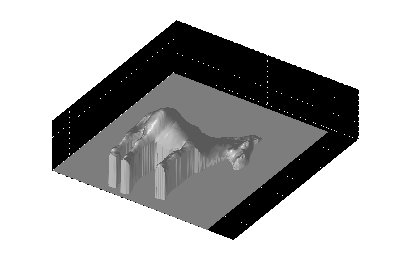
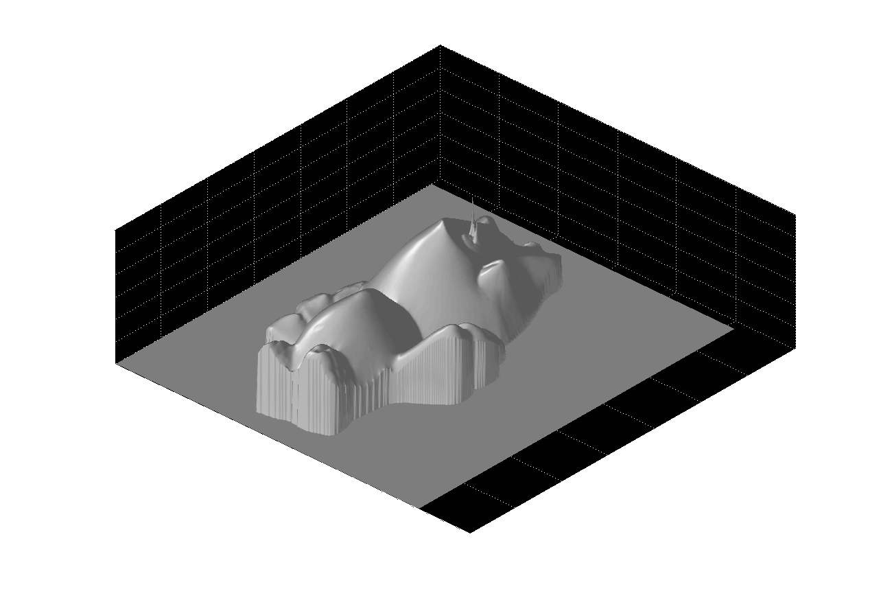
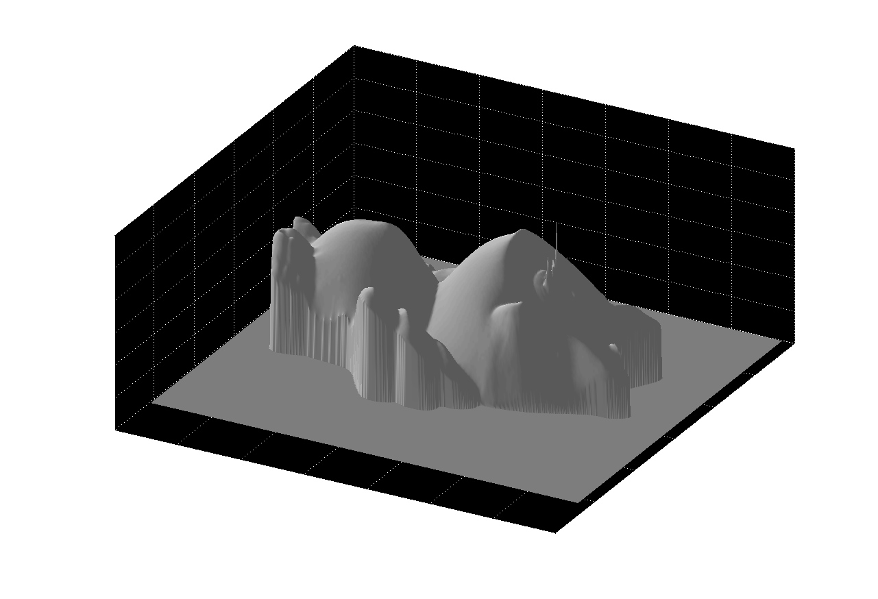
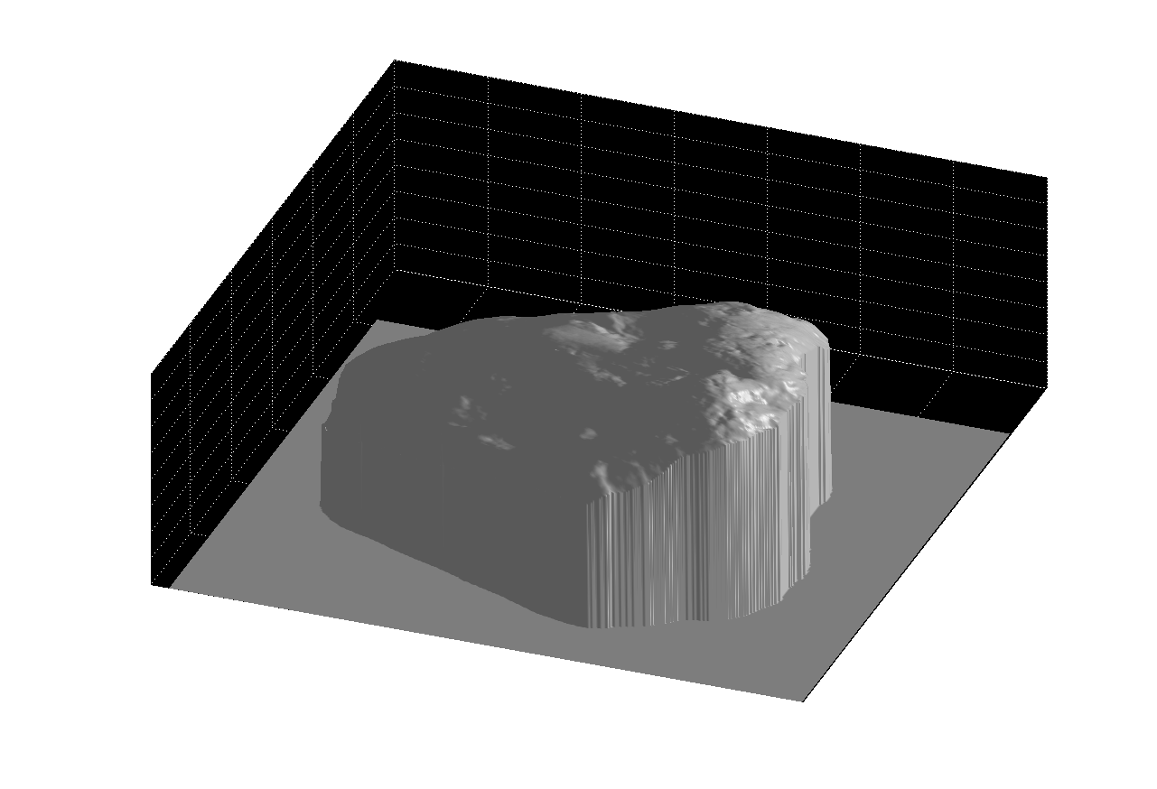
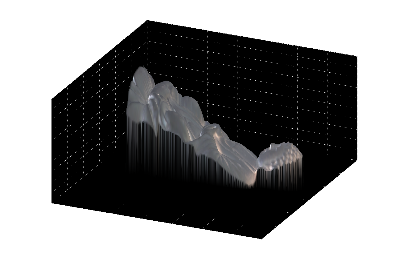
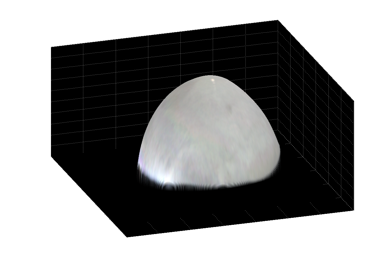
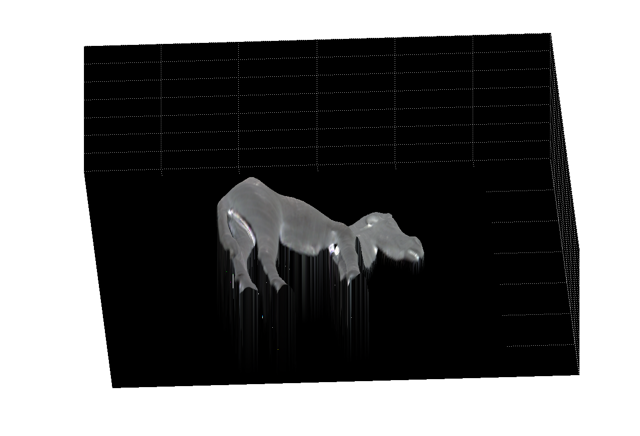
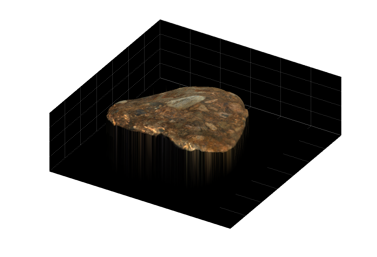
where z is a column vector containing all of the surface depths for the entire image. The surface depths were obtained by solving for z. 3D versions of the objects are shown in Figures 4 and 5.
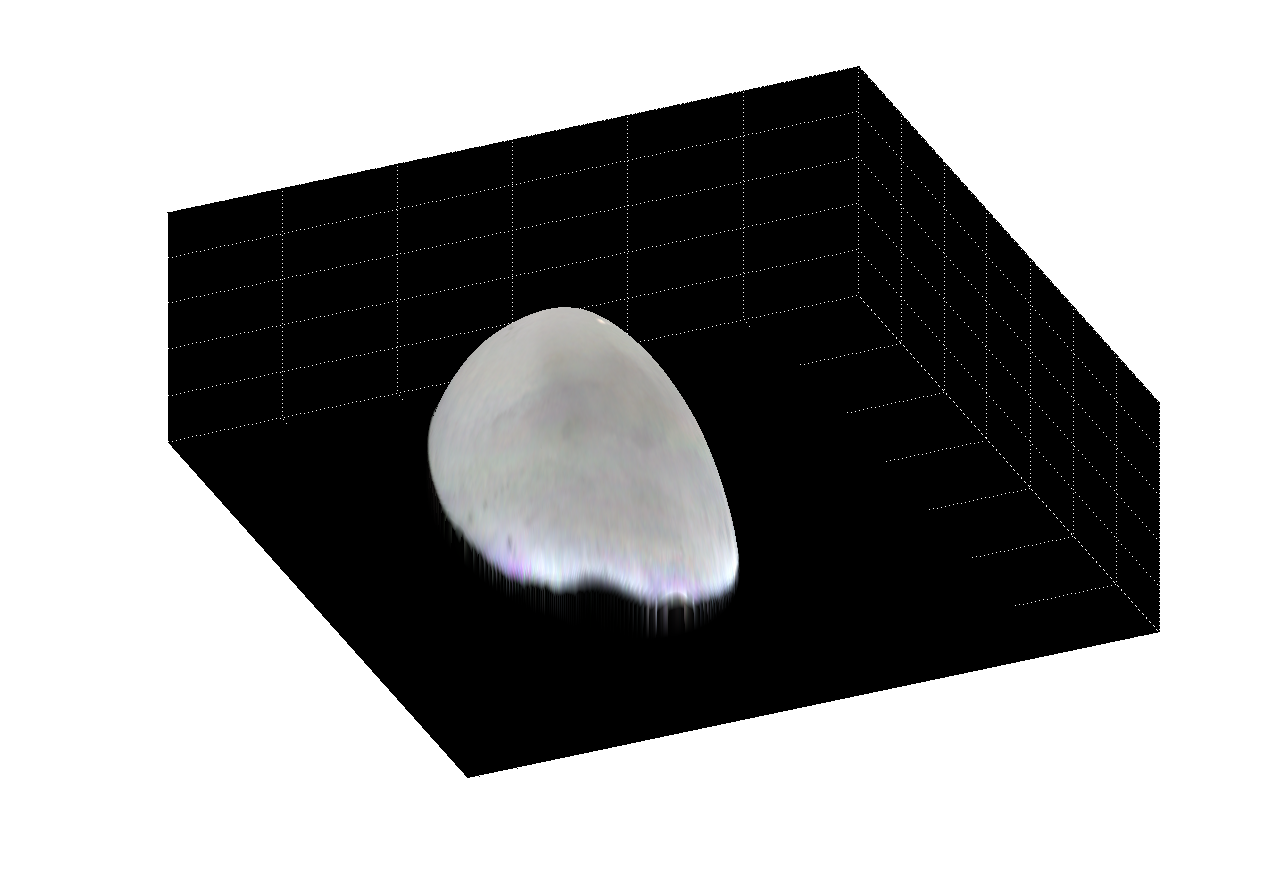
Figure 4: multiple views of the reconstructed surface without albedos
 |
 |
 |
 |
 |
 |
 |
 |
 |
 |
 |
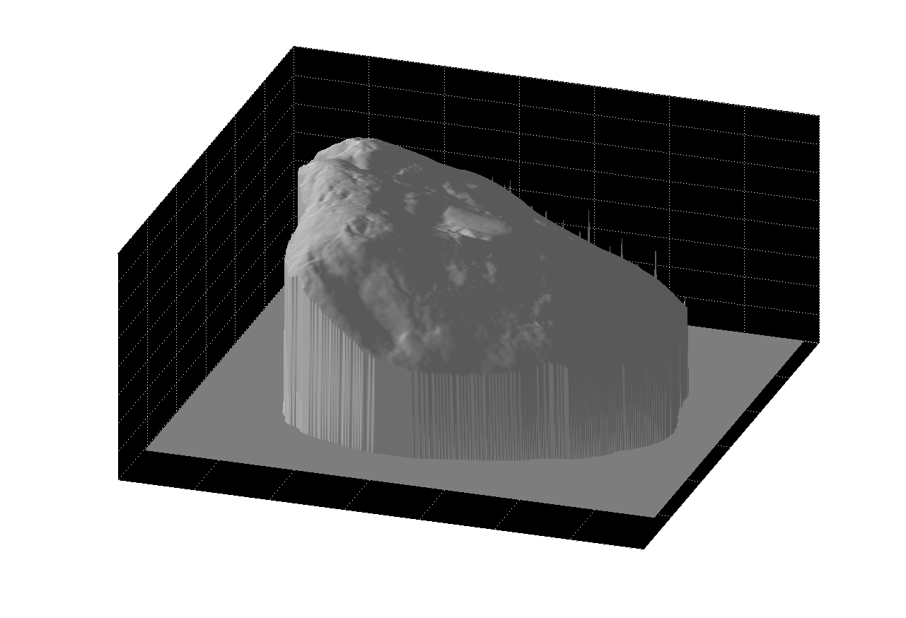 |
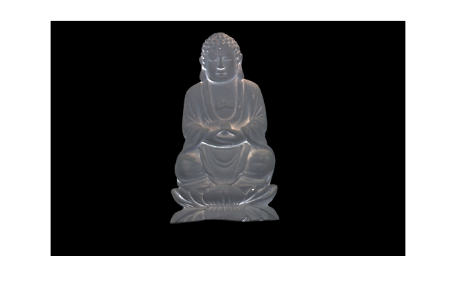
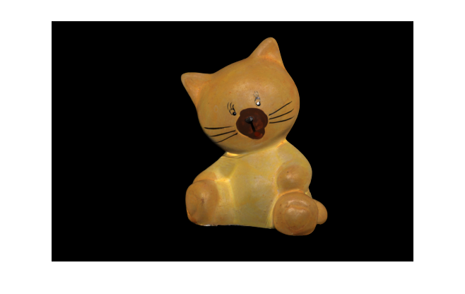
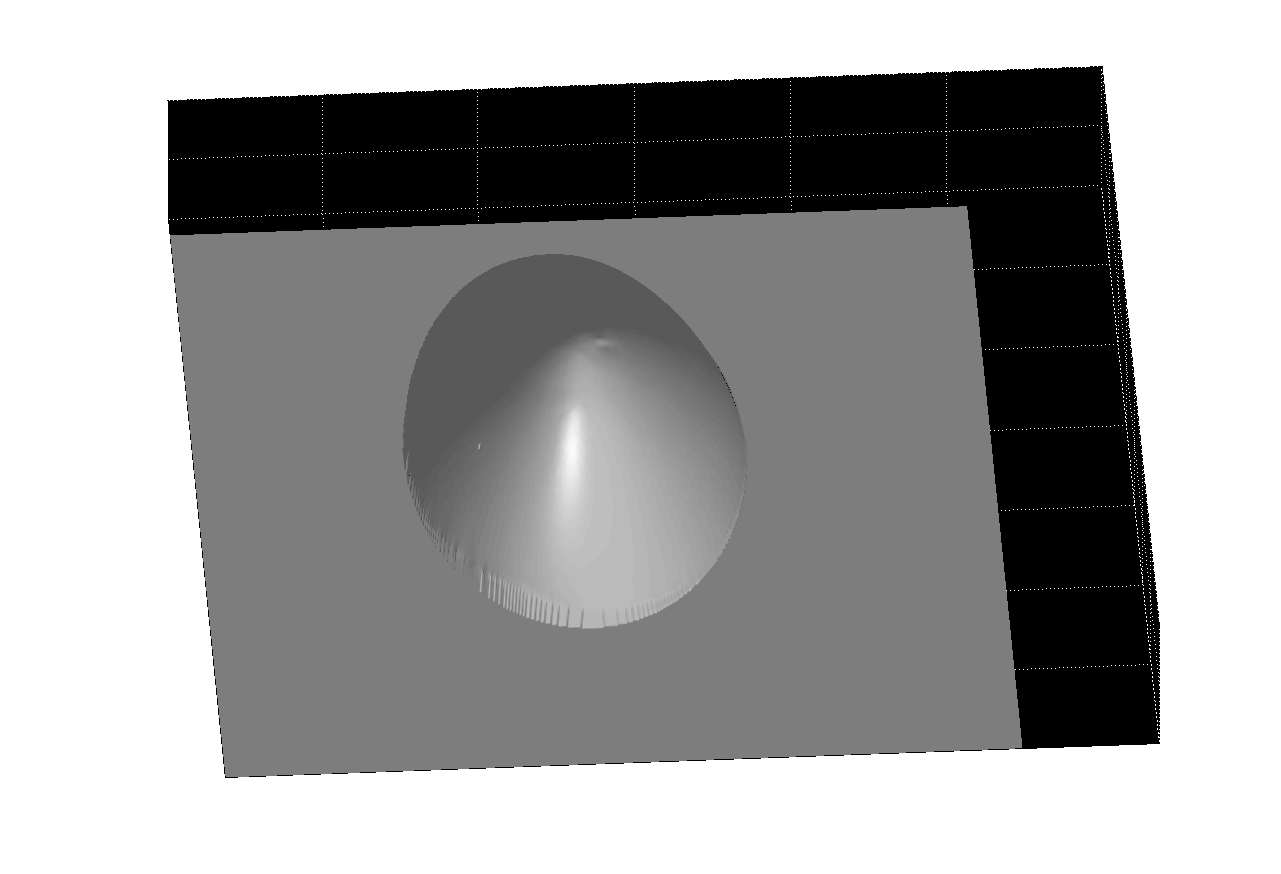
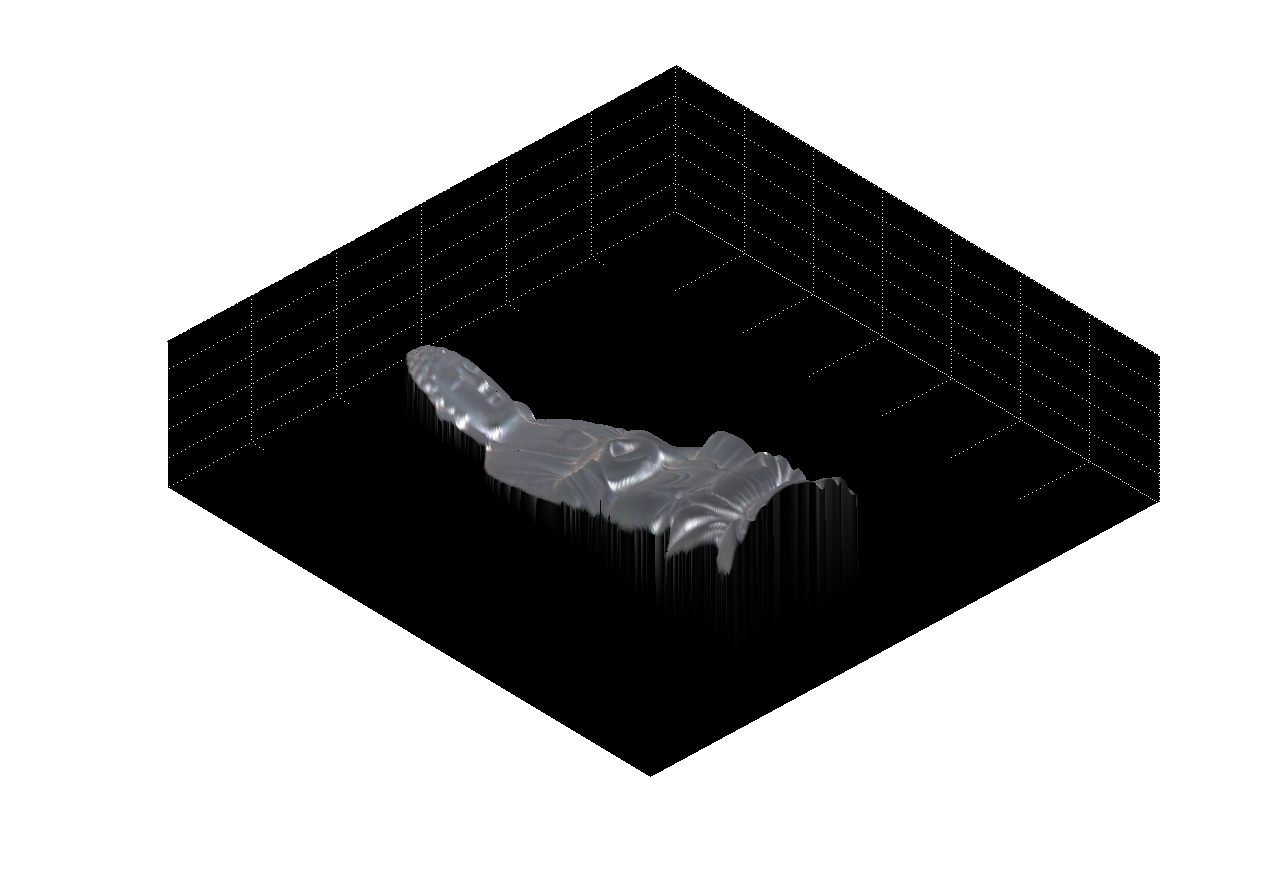
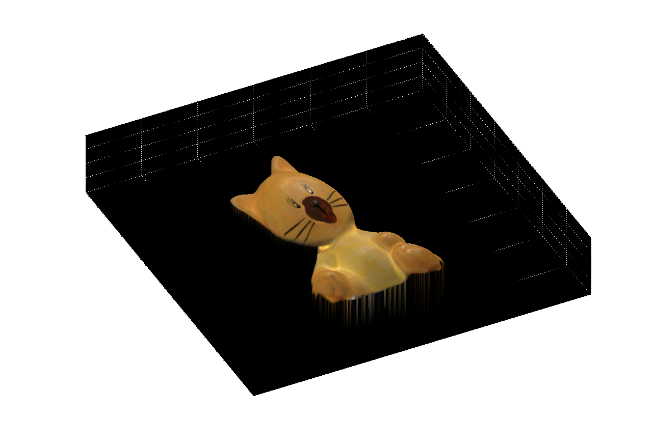
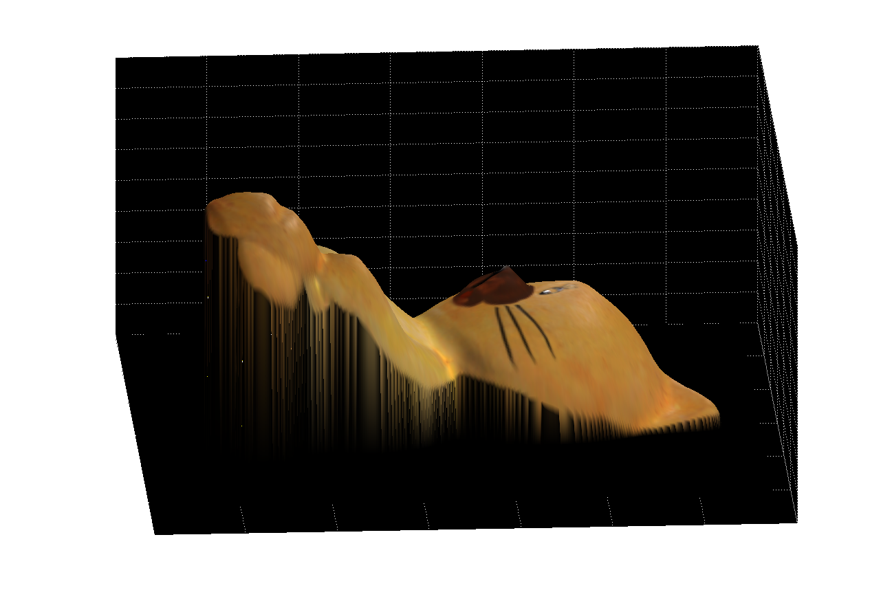
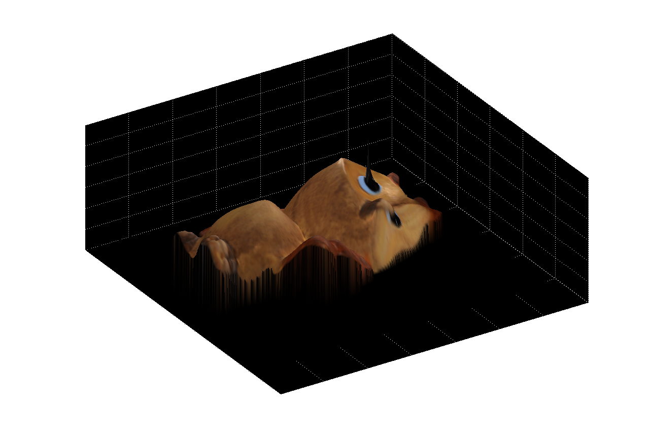
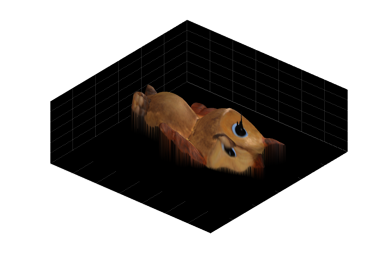
Figure 5: multiple views of the reconstructed surface with
albedos
 |
 |
 |
 |
 |
 |
 |
|
 |
 |
 |
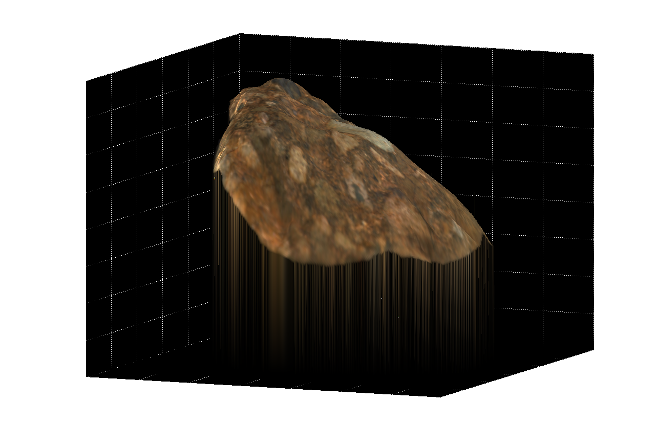 |
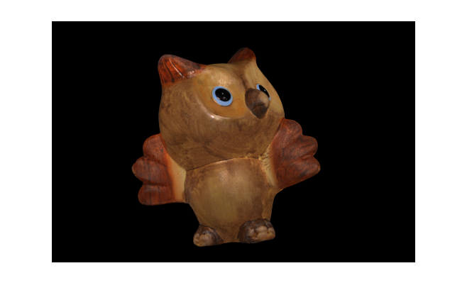
In general, the results were very good. However, the algorithm(s) implemented are not perfect. An interesting example of obvious error can be seen in the owl’s eye. Because it’s black, not much light intensity information can be gathered from it, and the surface spikes in this location.
imageResults/ (directory)
Holds all of the result images, organized by the folder each image was derived from (buddha, cat, gray, horse, owl, rock).
./*/*3DnoAlbedo1.tif
./*/*3DnoAlbedo2.tif3D images with no albedos shown, each shown at a different angle.
./*/*3DwithAlbedo1.tif
./*/*3DwithAlbedo2.tif3D images with (color) albedos shown, each shown at a different angle.
./*/*AlbedoMap.tif
2D image showing the (color) albedos.
./*/*QuiverNormals.tif
2D image showing the surface normal vectors as small arrows.
./*/*RGBNormals.tif
2D image showing the surface normal vectors encoded in RGB.
program/ (directory)
getBrightSpotOnSphere.m
Given an image of a chrome sphere (img), find the position of the center of the bright spot, assuming there is one.
getCenterOfSphere.m
Given a 2D image (img) of the mask of a sphere, return its center position (centerPos) in image coordinates, and radius in pixels.
getCompressedIndicesVec.m
Given an image mask, return xycoords, which holds the original x and y coordinates from the image.
getLargeSparseMatrix.m
Create the large, sparse matrices A and b which will be used to solve the system Az = b, where z wolds the depth values.
getLightingDirection.m
Given a normal vector (normVec), return the lighting direction vector (lightingVec). This assumes that the viewing vector (R) is orthogonal to the image plane (i.e., R = [0 0 1]).
getNormOnSphere.m
Given a 2D image position of a point on a sphere (position), the center position of the sphere (center), and the radius of the sphere (radius), return the normal vector at (position
getOneNorm.m
Calculate the albedo (kg) and N (the normal vector) on the surface at given a bunch of lighting direction vectors and a bunch of lighting intensities.
make3Dsurface.m
Given a compressed list of x and y coordinates, the image (so we can get height and width information), and Z, which is the depth, create a 3D image.
photometricStereo.m
This is the main program for Project 3. Simply give it the filename holding all of the chrome image filenames, and the filename holding all of the images, and the program takes care of everything. Figures are automatically shown for all of the required portions of the assignment (and then some). kg, N, and img3D are the albedo map, the surface normals, and the 3D image respectively.
readimages.m
Open the images indicated by the textfile whose name is passed in. Return an array of them.
show3Dsurface.m
Show the 3D image with the 2D picture plastered over it.
showQuiverImg.m
Display the normal vectors using the quiver function. The arrows will be spaced s pixels apart.
psmImages/ (directory)
The directory of images obtained from the project website.
readme.txt
Includes a list and an explanation of the directories and files.
report.doc
report.html
You’re reading one of these.
[1] Woodham, Robert J. “Photometric method for determining surface orientation from multiple images.” Optical Engineering. Vol 19, No.1. Jan/Feb 1980. Available online at http://www.cs.ubc.ca/~woodham/papers/Woodham80c.pdf
[2] Hayakawa, Hideki. “Photometric stereo under a light source with arbitrary motion.” Journal of the Optical Society of America, 1994. Available online at http://pages.cs.wisc.edu/%7Ecs766-1/projects/phs/hayakawa.pdf
[3] Forsyth, David A., Ponce Jean. “Computer Vision - A Modern Approach” © 2003 Pearson Education, Inc (Prentice Hall), Upper Saddle River, New Jersey 07458.
[4] Basri, Ronen, David Jacobs, Ira Kemelmacher. “Photometric Stereo with General, Unknown Lighting.” International Journal of Computer Vision. © 2006 Springer Science + Business Media, LLC. First online version published in June, 2006.
[5] Seitz, Steven. “Computer Vision (CSEP 576), Winter 2005 - Project
3: Photometric Stereo.” Available online at http://www.cs.washington.edu/education/courses/csep576/05wi/projects/project3/project3.htm