Chris Hinrichs
CS 766 Project 3 report.

Compiling and running requirements

This project was done in Matlab, so all stages of processing were done by Matlab scripts. Running them requires Matlab.

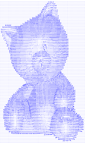
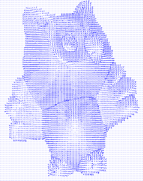
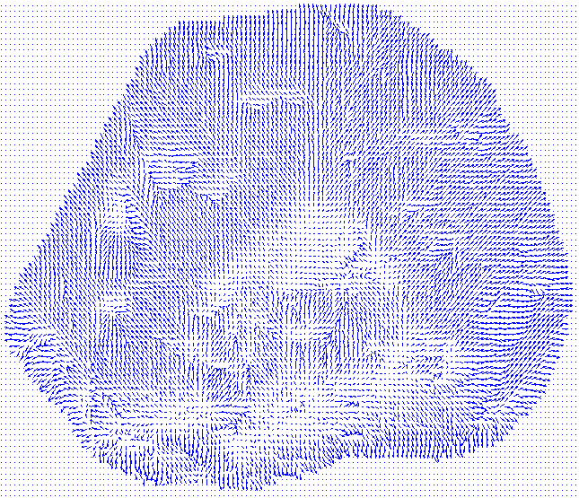
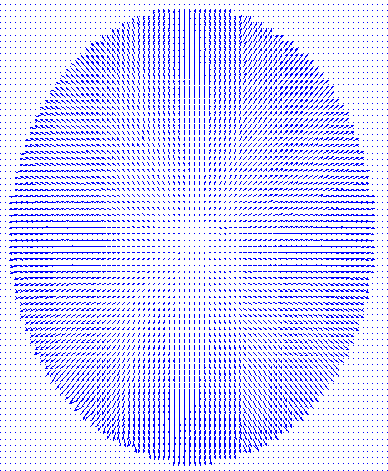
The Matlab command to display the surface normals is:

X = 1:3:512;
Y = 1:3:340;
dY = 340:-3:1;
quiver(X, dY, normals(Y,X,2) .* MASK(Y,X), -normals(Y,X,1) .* MASK(Y,X))

• get_L.m
  • Take a number in the sequence of chrome images, get the chrome image matching that number, find its highlight centroid location, calculate a surface normal from that, then double the angle between that normal and the incident vector to get the Lighting vector. This assumes that the incident vector is directly towards the camera under orthographic projection.
• get_MASK.m
  • Take the name of one of the sequences of images, e.g. 'owl', and get the mask for that sequence.
• get_normals.m
  • Take the name of one of the sequences of images, e.g. 'owl', and get the surface normal and albedo at every point on the image by solving the equation 1 for the normal vector n scaled by the albedo, for each pixel individually. Returns albedo and unit surface normal for each pixel.
• color_albedo.m
  • Given a surface normal for each pixel in a sequence of images, and the lighting vector for each image, solve the equation 2 for each pixel, and for each color channel in the sequence of images.
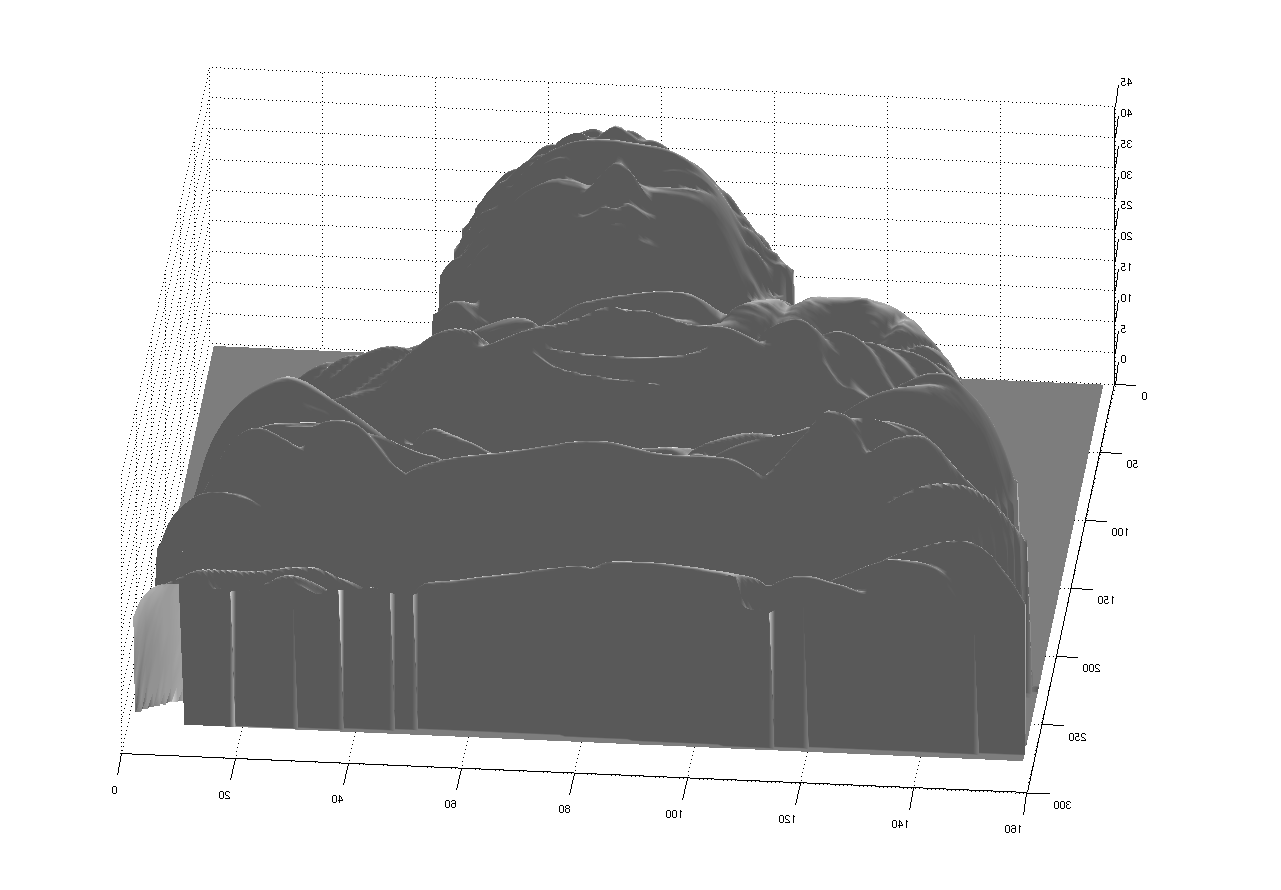
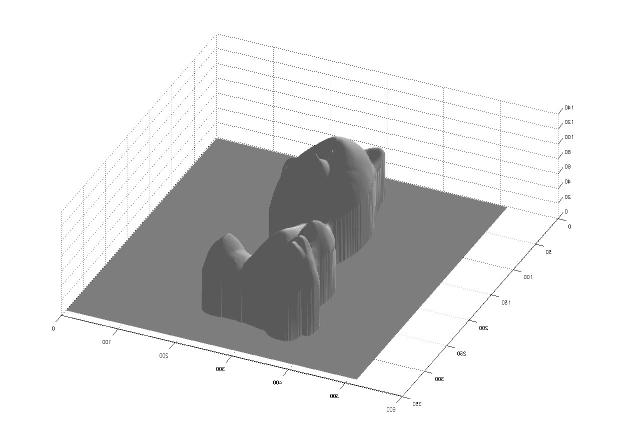
• get_depth.m
  • Given a set of normals, use the ratio of x and y tilt of each normal to solve the relative depth of the pixel to the right and below the current pixel and ground border pixels to have 0 depth.

Algorithms

Every stage of this work proceeded by setting up a system of linear equations describing the desired quantity in terms of known quantities, and solving for the desired quantity. In some cases, coefficients too close to 0 resulted in matrices with rank deficiency, (below some tolerance level,) so lower bounding coefficients to some epsilon prevented this without negatively impacting the quality of the resulting normals.

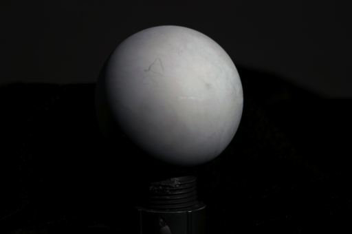
When finding the lighting incident vector, the centroid of the highlight region was found by taking the sum of the chrome ball image along each direction, (height and width,) and finding the range of values greater than half of the maximum value, then taking the mean of pixel indices in each range, giving the centroid of the region.

The radius of the chrome ball was found using the MASK image provided by taking the height and width of the non-zero region of the MASK, and averaging them. The height and width were found to differ by only 1 pixel.

An important innovation in finding the depth values is that the pixels whose neighbors were not part of the mask should be implicitly set to 0. This means that the neighbor of z_ij should be set to 0. This is achieved by simply setting the coefficient of zij in the array to 1, and leaving all other coefficients equal to 0, which implicitly constrains the neighbors of zij to be 0 without further altering the structure of the array.

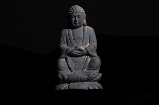
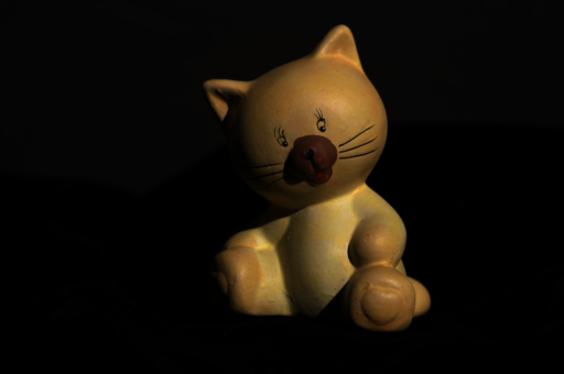
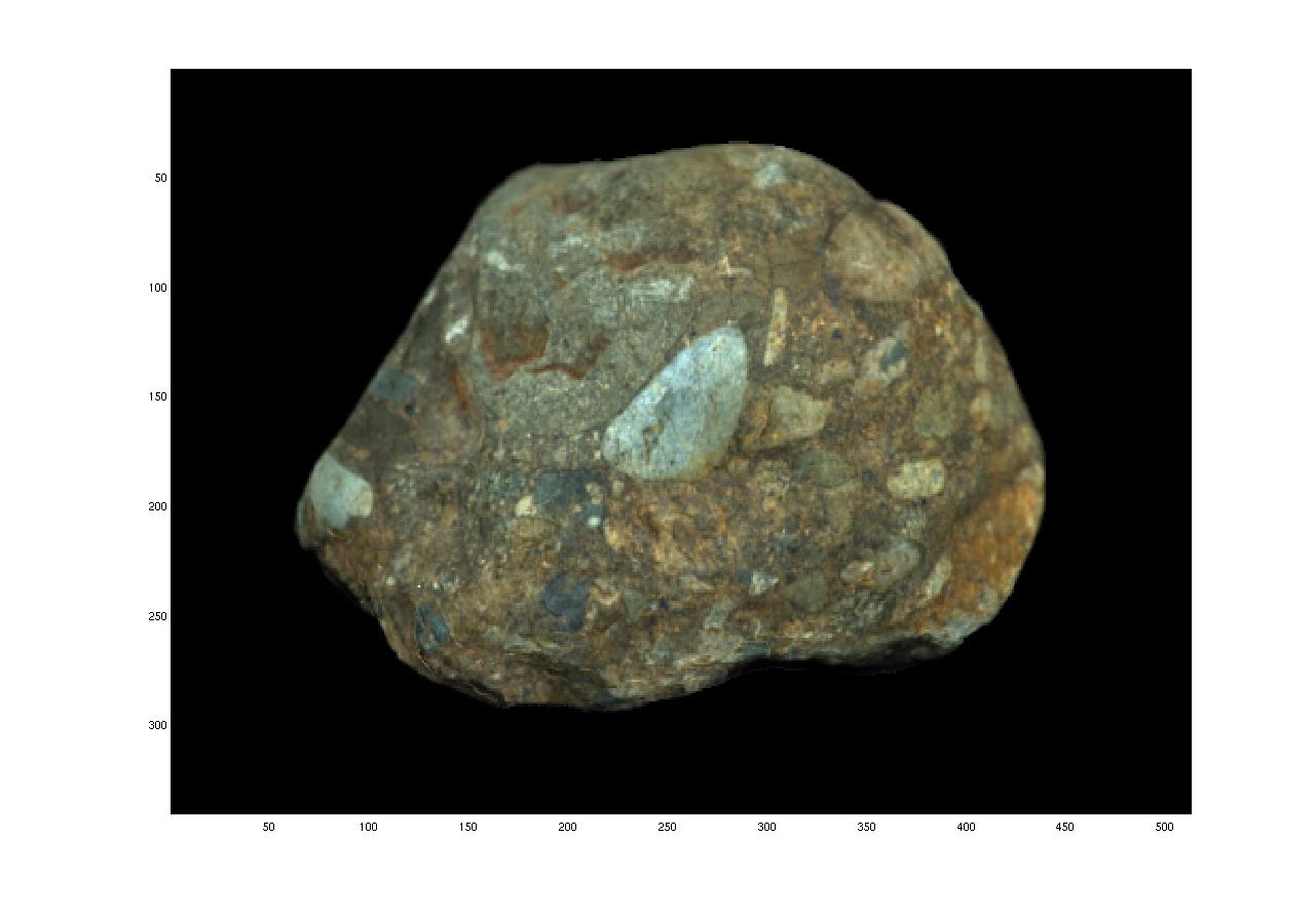
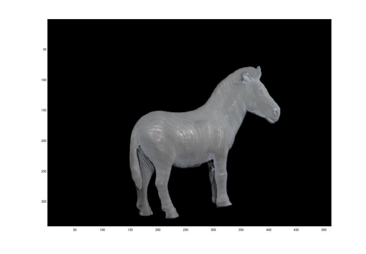
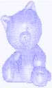
Results

The reference images looked like this:
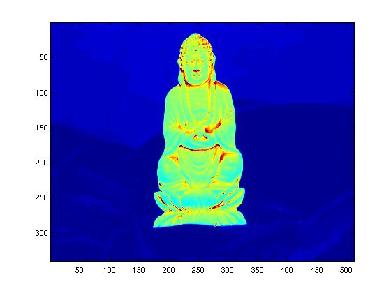
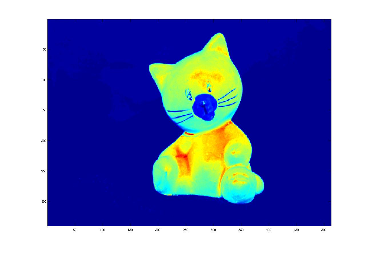
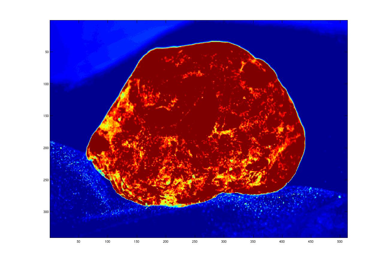
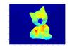
The albedo values as false-color images looked like this:
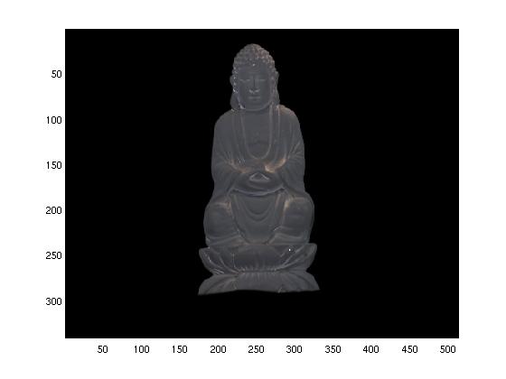
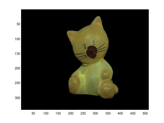
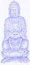
The color-albedo images looked like this:
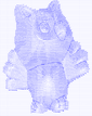
The surface normals looked like this:
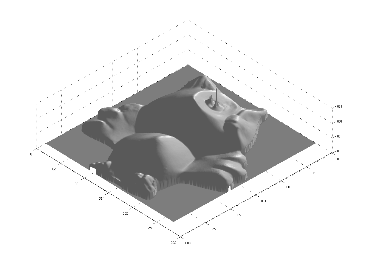
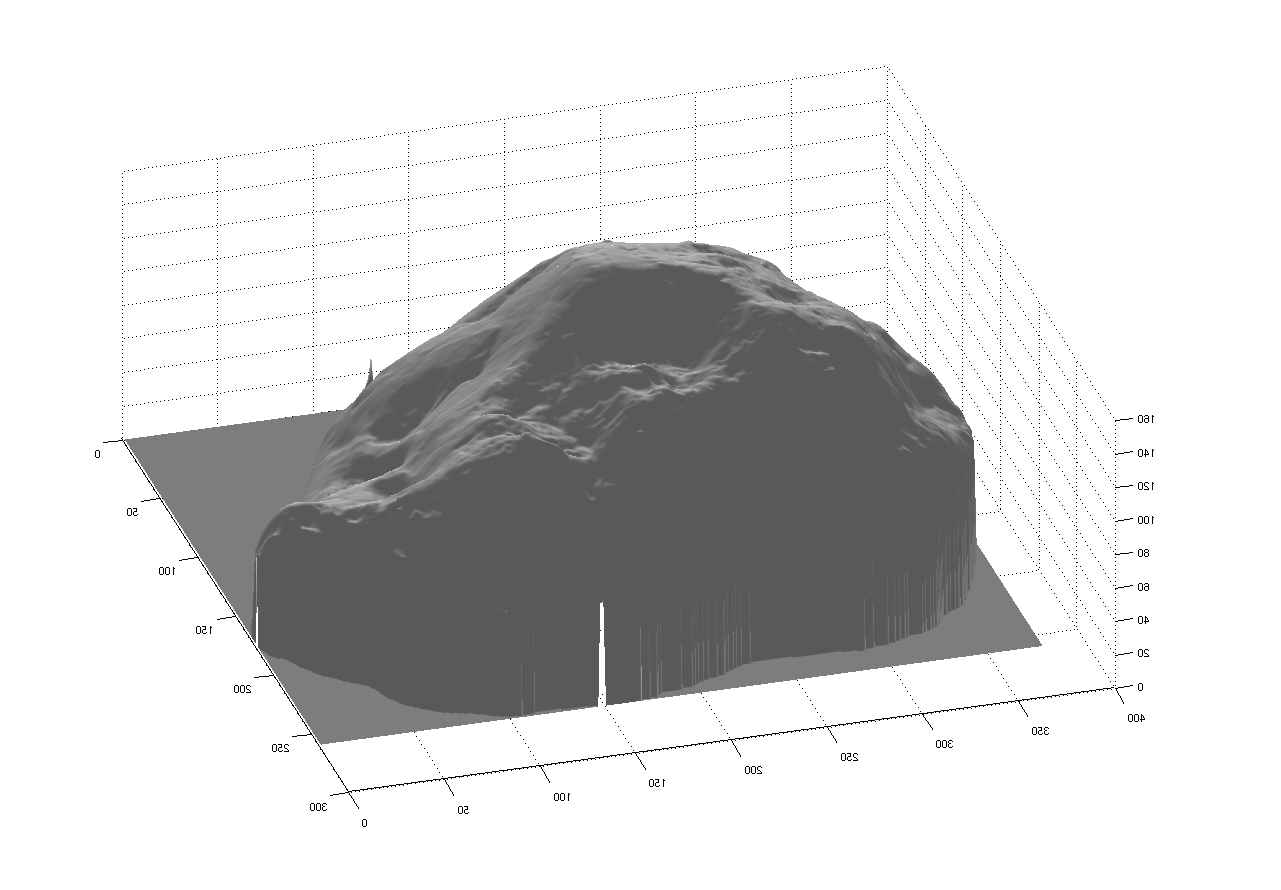
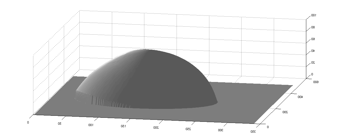
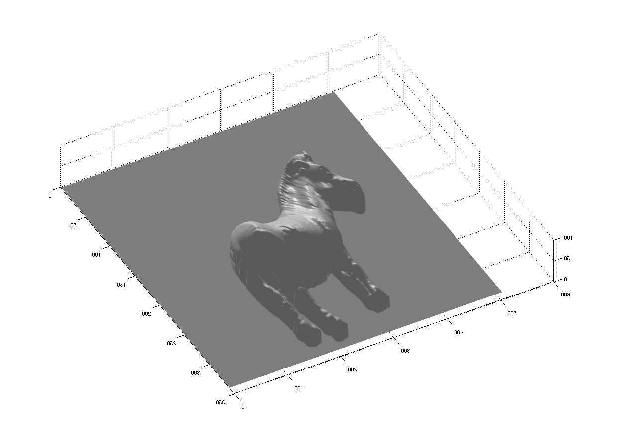
The pixel depths, represented as images looked like this:

The light vectors for each image in the series was determined by my program to be:

   0.4973    0.4662    0.7317
   0.2480    0.1323    0.9597
  -0.0416    0.1747    0.9838
  -0.0893    0.4465    0.8903
  -0.3170    0.5072    0.8014
  -0.1037    0.5581    0.8233
   0.2818    0.4267    0.8593
   0.1056    0.4386    0.8924
   0.2126    0.3353    0.9178
   0.0904    0.3370    0.9372
   0.1250    0.0417    0.9913
  -0.1391    0.3681    0.9193 

0.403259     0.480808     0.778592
0.0982272     0.163712     0.981606
-0.0654826     0.180077     0.98147
-0.127999     0.431998     0.892745
-0.328606     0.485085     0.810377
-0.110339     0.53593     0.837021
0.239071     0.41439     0.878138
0.0642302     0.417497     0.906406
0.12931     0.339438     0.931698
0.0323953     0.340151     0.939813
0.0985318     0.0492659     0.993914
-0.16119     0.354617     0.921013 

Discussion of results

A few things deserve notice. First, most of the light vectors agree with the given vectors, but in a few cases they diverge markedly, especially in row 2, column 1. This is a bit surprising, given that the level of detail captured from the images is very fine, when the light vectors are off by over 5 percentage points in several cases. The other thing to note is that the left column, which represents the horizontal component has greater errors on average, while the vertical components are all within 3-4 percentage points. One possible explanation for this is that the assumption of orthographic projection might break down, so perhaps the cases where the high-light was furthest from the camera's principal point were the cases with the greatest error. The chrome ball was centered in the image horizontally, but was off center vertically, (toward the top). This would tend to flatten the highlighted region horizintally, the further the sphere is from the horizontal plane. Whether this result is spurious or not, is not entirely clear from this.

Also, in the color albedo images, the redness seems somehow diminished. Since each channel was normalized separately from the other channels, it could be that the ratios of color channels in each image were not preserved, but the ratios of pixel values to all other pixel values were preserved. Under this interpretation, the maximum red pixel value could have been much larger than the maximum green or blue pixel value, causing the red albedo values to be reduced in the output. This effect could also be exaggerated by asymmetric sensitivity to different color channels in human eyes.

Also, in the owl depth image there are some notable outliers, which are probably due either to the surface normal having too small of a nz component, because a small absolute error there would result in a large relative difference in nx/nz, because this would almost result in a division by 0. A way to improve this would be to put a lower bound on nz values. Adding smoothing constraints to the matrix could be done, but from the images it appears that there is little improvement to be made, yet it would greatly increase the computational cost of solving for depth.

References