CS 766 Project 3 Report

Jake Rosin

10-22-07

Project Description

Construct a height field of a diffuse object using a series of images taking under different light sources. The vectors representing lighting direction can be estimated using the chrome ball method; from the lighting direction one can approximate surface normals for the object, and from these generate a surface map. Albedos and RGB-encoded normals were generated for all of the provided test objects, as were renderings of the height fields.

Implementation Details

The images provided were in TGA format; I had trouble opening these in MATLAB so I wrote a script in Python to convert them to TIFF files (this script is among my submitted files). All other code was implemented in MATLAB; the functions are described in the provided README. When I needed a way to convert from a cell array to a string, I found a freely provided MATLAB function here. All other code was written by me.

Algorithms Used

Estimating Lighting Direction: Lighting direction was calculated from the set of images taken of a chrome ball. The centroid of the sphere (on the image plane) was found by taking the average pixel position, weighted by the saturation of each pixel. Black areas outside the mask were weighted 0 and thus disregarded; white areas within the mask were given weight 1. Border pixels were weighted in (0,1) linearly with saturation. This approach assumes the value of a mask pixel is directly related to the proportion of the pixel which is occupied by the chrome ball.

The radius r was derived as half the height of the longest column of pixels within the mask (with border pixels again being valued in (0,1)) averaged with half the width of the longest row within the mask. Under this computation r = 119.497 pixels.

We estimate surface normals at a given point as follows. The point in question is represented as (x,y) on the image plane, with the origin at the sphere's centroid. For the chrome ball application the point is determined as the centroid of the reflected light (again, a weighted average of pixel locations, although all pixels with value < 0.5 - or < 128 for an integer-valued mapping – were assigned weight 0). The values (x,y) are the first two coordinates of a vector from the sphere's center to the point in question. This vector by definition has length r:

r = sqrt( x^2 + y^2 + z^2 )

r^2 = x^2 + y^2 + z^2

z = sqrt( r^2 – (x^2 + y^2) )

We can thus calculate a value for z, completing the vector. Scaling it to a unit vector gives the normal n.

We then make the assumption that all light rays travel in parallel from the image plane to the camera lens, and all such rays are perpendicular to the plane themselves. This gives us the vector of light from the surface point to the camera v = (0,0,1). From these two values we calculate the vector from the point on the sphere to the light source using the equation from the 10/4 lecture slides:

l = 2(n · r)n – r

Under another assumption – that rays from the light source travel in-parallel before striking objects in the scene – the vector l defines the direction from which light is striking every point in the scene. By repeating this procedure from normal generation on for each chrome ball image, a matrix of light directions can be derived:

L = [ l1x l1y l1z ]

[ ... ]

[ lNx lNy lNz ]

The values I calculated for this matrix differed slightly from those in the provided file lights.txt.

For the most part the by-component difference is small (< 0.06), although a few major discrepancies are apparent (compare the x component of the second light vector). The differences may have resulted from any stage of the light estimation process but I suspect they result from the process of estimating reflection centroids, since it strikes me as the greatest source of possible inaccuracy.

Surface Normals: The objective function for generating surface normals is given in the project assignment. It assumes a diffuse object, so results will be skewed for objects with non-negligible reflectance. A modified version of the objective function – the one used by my code – is shown below.

Q = Σ_i (w*I_i – w * L_i * g )^2

We define I_i as the light intensity at the pixel being considered in image i, and L_i as the ith row in the matrix L (defining the lighting direction in the ith image). For this step, and finding the albedo map, I only considered the object pixels which were fully inside the mask (i.e., the mask pixel had a value of 1). Pixel intensity I_i is taken from a grayscale version of the image. g is the term to be derived, representing the albedo k_d multiplied against the normal n. After g is estimated we can derive the normal by scaling to a unit vector.

The value w represents a weight on based on pixel intensity. The various weighting functions used are discussed in their own section below.

Color Albedo: In my implementation color albedo is found by a straightforward implementation of the equation given by the project assignment. No significant changes were made. With I_i representing the pixel intensity for image i in the color channel currently under consideration, albedo k_d is defined as:

Surface Fitting: The assignment description describes a method by which we construct vectors on the object surface formed by neighboring pixels on the height map. By definition any vector on the surface of an object will be perpendicular to its normal. We use this to our advantage, forming the equations

n_x + n_z(z(i+1,j) – z(i,j)) = 0

n_y + n_z(z(i,j+1) – z(i,j)) = 0

...with n representing the normal at pixel (i,j), and z(x,y) being the height of the surface under pixel (x,y). These equations can be represented as a matrix multiplication, making least-squares optimization possible in MATLAB. We form the equation Mz = v as follows.

M is a [#pixels*2, #pixels] matrix. Each pair of rows represents one pixel (i,j) using the terminology from the equations above – two rows are used because two equations are derived from each pixel. The columns represent image pixels as well. For the kth pixel, let us define its rightward neighbor as pixel k+1 and its upward neighbor as pixel k-c (noting that in MATLAB format moving up in the image matrix requires decreasing the row number), with c being the number of columns in the image. Within matrix M, the equations above are represented in rows 2k and 2k+1. We set:

M[2k, k] = -1 * w * n_z

M[2k, k+1] = w * n_z

M[2k+1, k] = -1 * w * n_z

M[2k+1, k-c] = w * n_z

All other entries in rows 2k and 2k-1 are set to zero. The term w above refers to the weight assigned to the pixel in our objective function; it is calculated based on the grayscale albedo at pixel k. I noticed that the calculated albedo was unnaturally dark in places corresponding to areas of the object which fell into shadow for most of the input images (examples can be found in the section for albedo results). I also assumed (though I didn't notice any specific examples in the data set) that highly reflective areas of the image will appear very bright in the albedo map. Specific weighting functions used are discussed in their own dedicated section.

v is a vector of length #pixels*2. Each pair of values represents one pixel (i,j). For the kth pixel we set:

v[2k] = w * n_x

v[2k+1] = w * n_y

It should be clear that if Mz = v, then z is a #pixels-length vector. Given the pair of equations which began this subsection, the kth entry in z represents the height of the object under pixel k. Setting a particular height for a single image pixel k may be desirable; this can be accomplished by adding a row r to M and v, setting M[r,k] = 1 and v[r] to the desired height.

We can also include smoothing terms in matrix M. For this we add a row for each pixel, making a matrix of size [#pixels*3, #pixels]. We calculate the weight w2 based on the grayscale albedo at pixel k, and set the following:

M[#pixels + k, k] = -2*w2

M[#pixels + k, k+1] = w2

M[#pixels + k, k-c] = w2

We keep the corresponding entries in v set to zero. This has the effect of introducing the constraint that the height of each pixel is the same as the pixels above and to the right of it – or, more accurately, that:

2z(k) = z(k+1) + z(k-c)

For most objects this constraint is incompatible with an accurate surface map. More information is available in the section on weighting functions. One final note: fixing the surface depth for all pixels down to the addition of some constant C, the smoothing term will tend to set C such that the average depth is around 0. This makes setting an explicit height for a particular image pixel somewhat unnecessary.

Normal and Albedo Results

Normals were mapped to RGB values by assigning x to R, y to G and z to B. However, the image is not rendered immediately due to the fact that pixel values range in [0,1] and any component of a unit vector may be in [-1,1]. I therefore scaled x and y to ensure that all possible values had some equivalent rendering. z is not scaled, as at no pixel of the object does the normal vector point away from the camera on the z axis (its value is always within [0,1]).

R = (x+1)/2

G = (y+1)/2

B = z

Intuitively one can understand “reddish” areas as having a normal pointing downward and to the right (i.e., having a positive x component, a negative y component and a z component of 0). “Greenish” areas have normals pointing upward and to the left. “Bluish” areas have large z components and x and y components which are close to being equal.

Compare below the RGB-encoded normal map for the image buddha.tga as generated by my implementation, and the one provided on the project website.

---------

On the left is the normal map produced by my program; on the right is the reference image. My image appears to have more prominent red and green areas, which may represent exaggerated x and y components of the calculated normals. On the other hand it may simply be an artifact resulting from different RGB encodings being used in the two images.

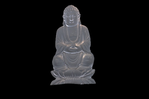
Albedos represent 3-channel color information, so they can be rendered directly without any conversion. Compare below the albedo map for buddha.tga produced by my implementation with the map provided in the psmImages directory.

---------

On the left, the albedo map produced by my program; the reference image is on the right. The only differences (aside from border pixels being omitted from my rendering) are found in the center of the Buddha's forehead and on the right side of the platform he is kneeling on, both small (2 by 2 pixels) areas brighter in the reference image.

Due to the negligible difference between the two images shown above I consider the results up to this point to be an unqualified success. The complete set of normal / albedo maps is available in the concluding images section; I unfortunately lack reference images for most of the objects presented.

Surface Map Results

I noticed a few oddities in producing the surface maps. First off is that while the height differences between pixels appears to have the correct ratio (for the most part), their absolute values seem compressed. The image gray.tga, for example, depicts a sphere – one would expect the height difference between the edge of the sphere and the center (of our 2D image representation) to be equal to the radius. Instead, I found it had a height of around r/2. Renderings for other images appeared similarly compressed. Scaling the z axis compensated for this problem when the images were being rendered with surfl.

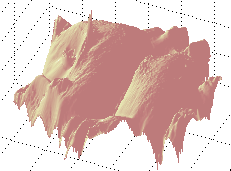
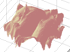
Surface map renderings were where the difference between my calculated light vectors and the provided ones had the most apparent effect. Consider the two renderings of buddha.tga below:

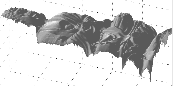
Above, the rendering produced when normals were calculated based on the light vectors estimated by my implementation. Below it, the rendering when the light vectors were read from the provided lights.txt.

Details seem to be slightly distorted in the rendering using my light vector information. This is especially apparent in the Buddha's facial structure – at least from this angle - but other angles showed that the folds in his robe (for example) were exaggerated in the top rendering. All other renderings presented in this report were made using my estimated light vectors.

The other hiccups I found in the surface maps are all best exemplified by a single image, and are thus discussed in the concluding images section.

Weighting Functions

The most obvious weighting function assigns a weight of 1 to every input. This was implemented as a baseline for comparison. The project assignment suggests a weighting function where w = I, the intensity of the given pixel, but also cautions that this has the drawback of overweighting saturated pixels. I skipped this function and implemented the suggested fix: reusing the weighting function from assignment 1. All normals were generated using this hat function to determine weight; it is defined as:

if (I < 0.5)

w = 2*I

else

w = 2*(1 – I)

I have included the scalar 2 in the result in order to allow for the following: both of these weighting functions are specific instances of a more generalized “monolith” or “Devils Tower” function, which takes two parameters – pixel intensity and threshold t – and is defined define as:

if (I < t)

w = I / t

else if ( I > 1 – t )

w = (1 – I) / t

else

w = 1

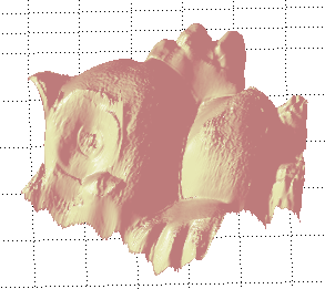
This gives equal weight to pixels within some middle range, but linearly reduces the weight towards zero as pixel intensity moves past the threshold towards shadow or oversaturation. All three functions were tested during the surface map generation step (the monolith function with t = 0.1). The results are shown below. I should take this opportunity to remark that all surface map renderings appear to be a horizontal reflection of the original source images. In fact they are vertically reflected; this is a result of the specifics of MATLAB's image processing and rendering functions, wherein images are indexed from the top left corner but surface plots are rendered with the origin in the bottom left.

------

From left to right: w(I) = 1, w(I) = monolith(I, 0.5), w(I) = monolith(I, 0.1).

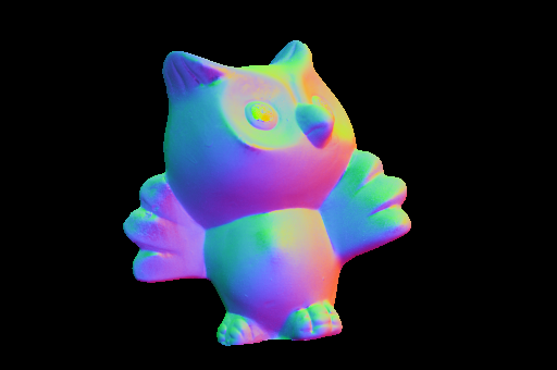
The difference made by the weighting function is most apparent around the owl's left eye. The unweighted rendering shows a visible pupil. As I do not have the object itself available to me I can only speculate, but it seems reasonable to assume that the owl's pupil was purely a coloring change and depth-wise was indistinct from its iris (in the source images iris and pupil together appear to form a dome).

Altering the weighting function does not appear to affect this artifact; instead, it has the effect of deforming the structure of the entire eye. Notice the bulge which appears below (relative to the page) the pupil in the two weighted renderings.

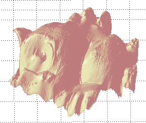
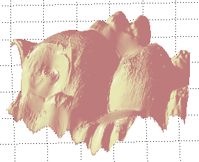
In my discussion of the matrices representing the surface map equations, I mentioned using a different weighting function for the smoothing term. I initially used the same weight (determined by pixel k) but found that this resulted in a severely distorted result, resembling nothing so much as a half-melted version of the correct rendering. In my current implementation I use the weight as determined by k but I scale it to reduce its effect relative to the surface vector equations, multiplying by the constant 0.1. Another view of the owl demonstrates the result:

------

The owls, in the same order as listed above, viewed from a different angle. Notice the spike emerging from the owl's cheek; in the source images this location was highly reflective, and oversaturated in a number of images.

The spike appears in all three images; furthermore it seems unaffected by the smoothing term. Using a constant larger than 0.1 may improve the smoothing effect, but I found that 0.1 was appropriate for another source image (the cat – unpictured). This suggests that simply setting some arbitrary constant to scale the smoothing function is inappropriate, and that different source images are ideally rendered using different scales for this constraint.

Additional Extensions

The weighting functions discussed above were implemented and tested. Since surface depth is defined by the generated normals, I may have had better luck testing different weightings on that stage of the computation – as mentioned above I used the hat function when determining normals. I also generated albedo and normal maps, and surface renderings, for all the provided test images.

Resulting Images

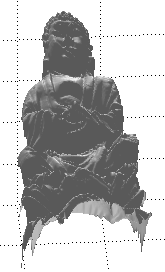
The Buddha: Albedos and normals were quite accurate compared to the reference images. There's nothing important to say about this image that I haven't said already.

-------

-------

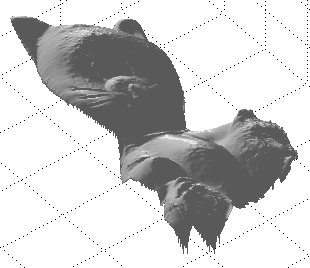
The Cat: The albedo map appears to glow almost unnaturally - this is probably due to the reflectance of the object's surface. The cat's left eye is inappropriately visible in the normal map; while the right eye appears it is much less subdued. This resulted in the bright spot over the left eye in the albedo map, and was itself undoubtedly the result of the reflection of the light source visible over the eye in cat.1.tga. The cat's paws show slight spikes in the renderings – these spikes were much more pronounced before the smoothing term was introduced into the surface map generation equations.

The close-up of the cat's face is provided to show the ridges formed by the cat's whiskers. From the source images I can't discern whether these whiskers represented actual depth or simply a color change.

-------

-------

The Gray Sphere: The results here are interesting. The normals appear correct, as do the albedos (aside from the dark crescent in the lower-left), but the rendered results do not even closely resemble the expected hemisphere. The degree of error here makes me skeptical of the other surface map results.

As a hack to enforce the proper structure for the shape I set the norm for all background pixels to (0,0,1) – a vector pointing directly at the camera. This has the effect of enforcing a “background plane” from which the hemisphere emerges. This constraint allowed the correct rendering to be produced – unfortunately it is not generally applicable, as it relies on the assumption that the border (the silhouette) of the image is at a constant depth. For most objects this is not the case; only the simplicity of the sphere and the fact that it's shape was known in advance made it possible.

With the background plane in place the hemisphere appears to be correctly rendered, meaning surface depth was correctly generated (aside from the bumpiness of the surface).

-------

-------

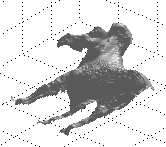
The Horse: The albedo seems reasonable for the most part – notice the bright lines apparent on its left legs (which are in shadow in a large number of source images). These artifacts are also apparent in the normal map.

The rendered version of the horse puts both sets of legs at the same depth. This result is obvious in hindsight but was not expected. A close examination of the source images shows that the junction between the horse's rear left leg and the its body is not visible from this angle. The normals therefore do not describe a surface which smoothly connects the more distant hind leg with the rest of the surface. Without this information, the surface map equations assume the leg is directly connected with the neighboring pixels.

-------

-------

The Owl: The distortion apparent in the normal map – at the owl's pupil and its right wing – is also apparent in the surface map (remember that the surface map is reflected, so look at the owl's left wing there).

-------

-------

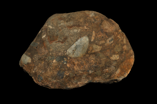
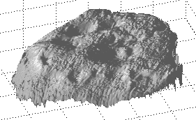
The Rock: This one turned out pretty well. Notice the shadowed areas along the bottom of the rock in the albedo map, and the corresponding errors in the normal map. Areas which do not receive good lighting in any source image (or even those which receive it in a minority) are frequently misrepresented in the resulting images.

-------

-------

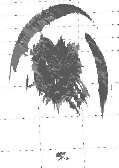
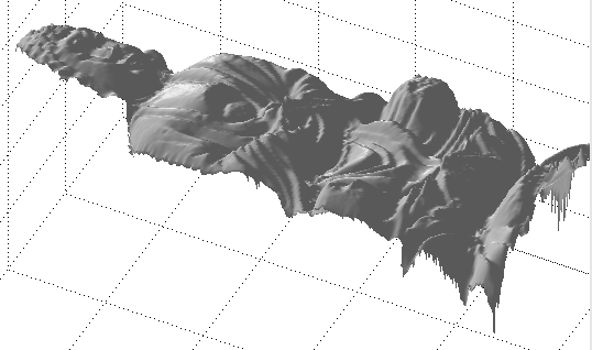
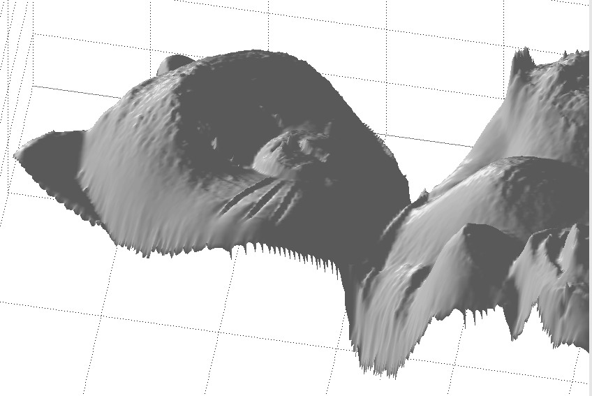
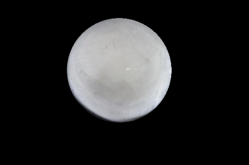
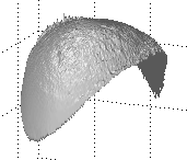
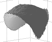
The Chrome Sphere: This last one was just for fun. I took the chrome sphere images, used to determine lighting direction, and applied the same surface map calculations to them. Since most of the equations assume a diffuse surface, I expected meaningless results (and got them). They look neat though.

-------

-------
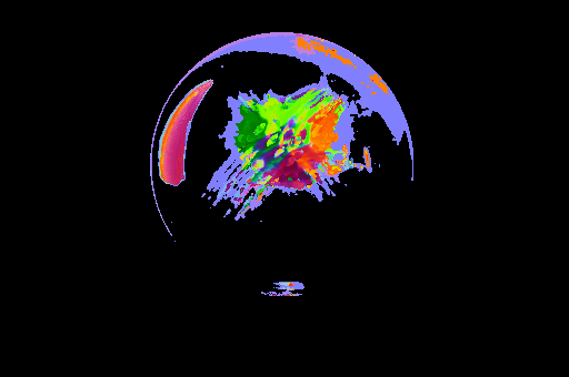
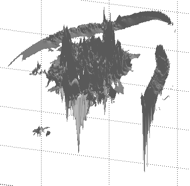