CS 766 Project 1: High Dynamic Range Imaging
by: Adam Bechle
Introduction
As the name implies, the goal of this project was to develop a high dynamic range (HDR) image. Typical images are 8 bits and have a dynamic range of 256 possible intensity values. On the other hand, an HDR image exhibits a greater range of brightness values than a single exposure can capture, allowing for both bright and dark regions of the image to be displayed. The basic premise of the HDR image is to determine the brightness information of the imaged scene based on multiple images taken at varying exposure times. This will result in a relationship between the 8 bit pixel intensity Zi,j, exposure time Δt, and the sensor irradiance at a given pixel Ei. This relationship is described in Equation 1, where g(Zi,j) is the unknown function known as the response curve of the sensor. The goal of the HDR project is to define this function and use it to develop an HDR image.
![]() (1)
(1)
Algorithm
There are multiple methods in which the response curve can be recovered. In the case of this project, the technique proposed by Debevec (1997) was followed. In this method, the response curve is found by minimizing the function given in Equation 2, which includes a form of Equation 1 in addition to a smoothing term featuring the constant λ and a hat weighting function w.
 (2)
(2)
In Equation 2, N is the number of pixels used in the solution as the basis of the response curve; P is the total number of exposures. To solve this relationship, the relationship is converted into a matrix multiplication resembling a least squares solution, with the lnΔt term being the constant. The response curve is recovered through an SVD operation. Once the response curve is found, is can be used in Equation 1 to solve for the sensor irradiance Ei, for each pixelin the image. An image composed of the sensor irradiances is known as the radiance map of the image. This radiance map has infinite dynamic range, which is our desired result. However, we cannot display an image with infinite dynamic range, so we must use the radiance map to create a tonemap, which transforms the radiance map into a viewable HDR image.
Implementation
The Debevec algorithm was coded in Matlab in order to solve for the response curve determine the radiance map. The main function is HDR_run.m, which loads the images, allows the user to select the points Zi,j, and calls response.m. The function response.m takes the points Zi,j, exposure times Δt and computes the response curve, g(Zi,j). Though Debevec provides a Matlab code for the response curve solution, I programmed my own to get a better handle on the problem. The functions are very similar, though some operations, such as translating the response curve, are different.
After response.m computes the response curve, it returns it to the main function HDR_run.m, which proceeds by calculating the radiance map of the image, Ei. Once the radiance map is computed, it is saved as a Radiance RGBE image in .hdr format by the Matlab supplied function hdrwrite.m, which is included in the Image Processing Toolbox of Matlab 2008a. The radiance map is then tonemapped in HDR Shop using the Reinhard HDR Tonemapping Plugin to create an image viewable on a standard computer monitor.
To run HDR_run.m, the following line should be written in the proper Matlab directory: HDR_run(image_rootname, n_start, n_end, dt, lambda), where image_rootname is the file rootname of the image series. I used AHDRIA to aquire my images, which names the files ‘AHDRIA_#.jpg,’ so the rootname would be just ‘AHDRIA_’. The variables n_start and n_end are simply the first and last image numbers that are to be processed. The variable dt is a Px1 vector containing the exposure times of each image, beginning with the image corresponding to n_start. Finally, lambda is the smoothing term, which I usually set to 1. The function will solve for and display the response curve, as well as save the radiance map to radiance.hdr.
Image Acquisition
The images for this project were acquired using a Canon Powershot A640. The program AHDRIA was used to remotely trigger the camera to take multiple images at one aperture (f/5.8) with varying exposures. The camera was placed on a tripod and most of the subjects were stationary objects, so image alignment was not necessary to remove motion.
Results
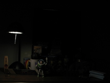
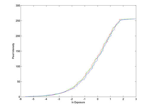
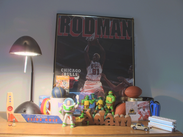
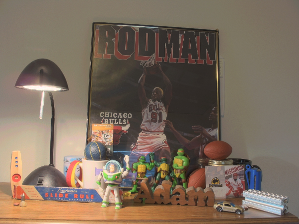
The HDR image developed for this project was taken of my desk at my apartment, with a low and high exposure image seen in Figure 1. The lamp on my desk was turned on, which provided intense light to most of the objects in its vicinity. However, the objects on the right of the image and the Dennis Rodman poster in the background were not well lit by the lamp, so they require a longer exposure time for viewing. A total of 17 images with exposure times varying from 1/2500 s to 15 s were used to construct a response curve, seen in Figure 2. The response curve has been shifted such that Z129 is zero for all three color channels, as suggested by Debevec. The response curve was used to generate the final tonemapped HDR image, shown in Figure 3. For the most part, the HDR image was a success and the image does a good job at making all of the objects visible.
The main issue I noticed in the image was with the contrast of Buzz Lightyear in the lower left quadrant. In the low exposure time images, he has decent contrast with his background, but in the tonemap, his right arm becomes less distinguished from the similar colored background objects. In retrospect, this is somewhat expected, as all of the objects in that region are similar colored and appear distinct in the original images due to variations in exposure so they become less distinguished when mapped in a HRD image.
The scene of my desk was also shot with artificial lighting provided by an overhead ceiling light. The HDR image is given in Figure 4. However, this image did not provide as good of image quality and did not use the HDR concept as much as the previous non-lit image since the entire image was more well lit. Also, an HDR of the third floor of the Engineering Centers Building is given in Figure 5, though it does not feature a very high dynamic range, as the only feature that is enhanced is the far window.
 |
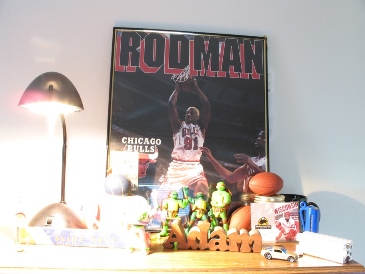 |
Figure 1: Short (1/80 s) and long (3.2 s) exposure images of my desk. |
|
 |
|
Figure 2: Response curve for Canon Powershot A640, with red, green, and blue channels represented by their respective color. |
|
 |
|
Figure 3: HDR image of my desk. |
|
 |
|
Figure 4: HDR image of my desk featuring artificial lighting from a ceiling light. |
|
 |
|
Figure 5: HDR image of the Engineering Centers Building |
|
Lessons Learned
Through this project, I learned a few things about photography and one important life lesson. This was my first experience with using manual controls on a consumer camera, so I learned how to set exposure and aperture. This taught me the difference these functions make in image quality. In addition, I utilized remote control of the camera, which turned out to be very convenient. I was already familiar with processing images in Matlab, so I was able to handle that well, but the whole algorithm implementation from a few equations was relatively new to me, especially composing and solving the response optimization matrix.
Finally, perhaps the most important lesson learned is to always be sure of project deadlines. I realized late Wednesday afternoon that the project was due on Thursday at noon and not Friday, like I had thought. Needless to say, this motivated me to work a little harder on finishing the project and has taught me to always double check when something needs to be done.
References
Debevec, Paul E., Malik, Jitendra. Recovering High Dynamic Range Radiance Maps from Photographs. SIGGRAPH 1997.
Reinhard, Erik et al. Photographic Tone Reproduction for Digital Images. SIGGRAPH 2002.