CS 776 Project 1

By Mikola Lysenko and Houssam Nassif

Date: September 25, 2008

Project Installation Instructions

Project implemented under Linux. If for some reason it can't run on your machine, we would be happy to demonstrate a session on one of our CS accounts.

We used GSL, which should already be installed on the lab machines.

OpenCV Installation

1. Download sources from:

       http://sourceforge.net/projects/opencvlibrary/
   

2. Extract files to local directory

       (eg ~/Desktop/OpenCV)
   

3. cd to local directory

       cd ~/Desktop/OpenCV
   

4. Make build directory

       mkdir ~/opencv/
   

5. Run configure script with build prefix

       ./configure --prefix=/YOUR HOME DIRECTORY/opencv
   

6. Install files

       make && make install
   

FFTW Installation

1. Download sources from:

       http://www.fftw.org/download.html
   

2. Extract files to local directory

       (eg ~/Desktop/OpenCV)
   

3. cd to local directory

       cd ~/Desktop/FFTW3
   

4. Make build directory

       mkdir ~/fftw3/
   

5. Run configure script with build prefix

       ./configure --prefix=/YOUR HOME DIRECTORY/fftw3
   

6. Install files

       make && make install
   

Building the Project

1. Extract project files
2. cd to project directory
3. Build program

       make all
   

4. Run the executable with some sample data:

       ./a.out < data/shutter.txt
   

5. Enjoy!

Shutter Time File Format Description

Just a set of values of image files with exposure times:

    image_file.jpg   0.1

Image files can be PNG, JPG, GIF, TIF, TGA. Exposure times are given in seconds.

Matlab Code

Since we are not using the gil library, we have to somehow write our output in a format that Matlab can process.

Here is the Matlab script:

load R.dat;
load G.dat;
load B.dat;

hdr = repmat(0, [size(R),3]);
hdr(:,:,1) = R;
hdr(:,:,2) = G;
hdr(:,:,3) = B;

rgb = tonemap(hdr);
imshow(rgb);

Taking Images

We took several images of six different scenes, using the PowerShot SX100 IS Canon camera. We used a tripod and manually changed exposures and pressed the shutter.

We implemented De Castro and Morandi's image alignment algorithm (Registration of Translated and Rotated Images Using Finite Fourier Transforms, IEEE Trans. Pat. Anal. 1987). The basic idea is to compute

$$max_{x} (f * g)(x)$$

where $*$ is the convolution. Since the best alignment is the one with the highest convolution, finding it amounts to maximizing the convolution score. This method uses cross-power correlation. We performed the Discrete Fourier Transform using FFTW library.

Assemble HDR Image

We implemented a program to take the captured images as inputs and output an HDR image as well as the response curve of the camera. We coded in C++, using the OpenCV and GSL libraries on a Linux platform.

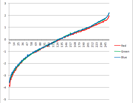
Figure 1 plots our camera's response curve for the three color channels. We can see that the three colors follow a similar curve, and that the curve is S-shaped. We computed the $g$ curve for every set of pictures we took (check the curves folder). The shapes of the six curves are similar. We only plot one of them.

Figure 1: Response curve.

We used Debevec and Malik's algorithm (Recovering High Dynamic Range Radiance Maps from Photographs, SIGGRAPH, 1997). To generate $g$ with large images, we randomly choose a subset of the pixels to perform Singular Value Decomposition on. The running time grew exponentially with the number of samples. We ran our experiments with $300$ to $600$ random samples.

Since we are not using the gil library, we have to somehow write our output in a format that Matlab can process. We can not generate the hdr file as gil does. Instead OpenCV generates a TIFF file. We can generate a HDR file using $8$ bits for every color channel per pixel, in the format discussed in class; or generate a separate file for every channel. Since our Matlab script works by combining the three color channel files, we include them as our recovered hdr files (check recovered_hdr directory).

Tonemapping

We used Matlab's tonemap functionality for tonemapping. Our C++ code outputs a radiance matrix that is read and processed by Matlab.

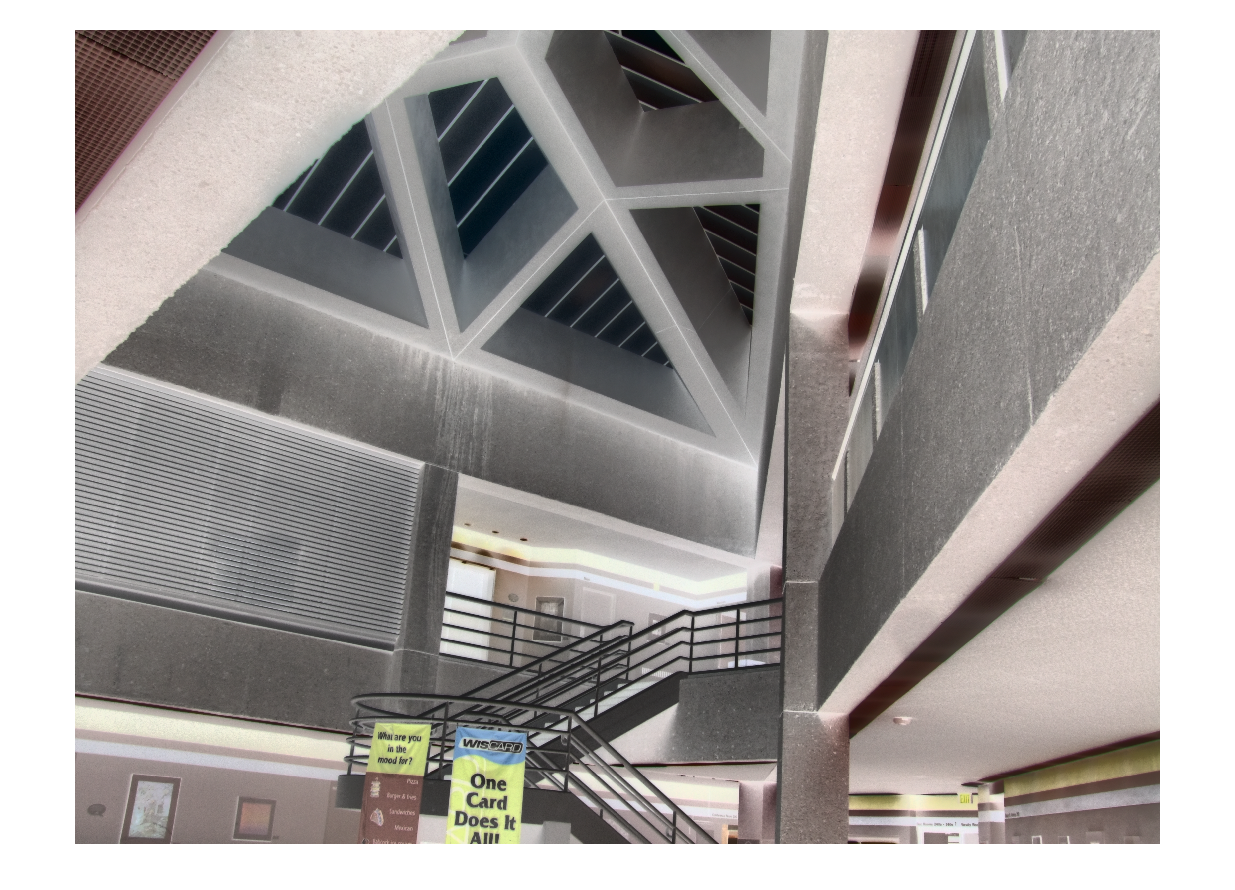
Figure 2 shows one of our recovered HDR images. The other five can be viewed in the hdr_images folder. The original pictures, with their shutter speed, are in the data folder.

The tonemapped images look dim. The color ratio should be adjusted. We did that by varying the AdjustSaturation and AdjustLuminance parameters. This improved the look of our images, although they still lack perfect color balance.

Figure 2: HDR image.

Bonus

We implemented image alignment, as discussed above. We also worked under Linux.

Authors Contributions

Mikola Lysenko researched Linux libraries and provided Linux support, researched and implemented image alignment, extracted the response curve and co-wtrote the HDR assembly code.

Houssam Nassif researched and implemented tonemapping, took the pictures, ran the experiments, performed HDR assembly, co-wrote the HDR assembly code and compiled the report.

About this document ...

CS 776 Project 1

This document was generated using the LaTeX2HTML translator Version 2002-2-1 (1.70)

Copyright © 1993, 1994, 1995, 1996, Nikos Drakos, Computer Based Learning Unit, University of Leeds.
Copyright © 1997, 1998, 1999, Ross Moore, Mathematics Department, Macquarie University, Sydney.

The command line arguments were:
latex2html report.tex -no_subdir -split 0

The translation was initiated by Houssam Nassif on 2008-10-02