Implementing Seam Carving for Image Resizing
| Moayad Alnammi | |
| alnammi@wisc.edu | |
| CS 766 Project |
The goal of this project is to implement the Seam Carving approach, apply it and analyze its effectiveness/limitations on different applications. Seam carving is a method for resizing images to a desired target size with the goal of preserving the contents of the image. Introduced by Avidan & Shamir [1],it is a content-aware procedure that supports reduction and expansion. A seam is simply a connected path of pixels that extends from top-to-bottom or left-to-right in an image. The procedure changes the size of an image by removing or inserting pixels that are part of the seam. The choice of which seam to alter depends on the content of the image and is reflected via the use of an energy function. This approach can also be used to amplify and remove certain objects in the image while retaining the original size. Furthermore, in the second paper by Rubeinstein, Avidan & Shamir [2], they introduced several improvements on the original, most importantly its application to videos.
In this report, I will detail my implementation of the project and the results I have obtained. The first part will cover the related work and project milestones achieved. Then I will discuss the components and their implementation in greater detail. Finally, we will conclude with contrasts, comparisons and limitations of seam carving relative to other common approaches.
Matlab code and GUI application can be found at the end of this page: here.
There are two common approaches to content-aware image retargeting: discrete and continuous. While discrete approaches manipulate individual pixels, continuous methods on the other hand perform a complete mapping of the source image to the target image. Both methods can make use of extra information and constraints to optimize their decisions (e.g. face detection, user supplied region selection, etc.). Known approaches include: Shift-mapping, scale-and-stretch, energy-based deformation, and nonhomogeneous warping. Each method suffers from certain limitations and perform better on some tasks over others. [3]
The following table summarizes the project milestones set forth in the proposal and the progress so far:
| Date | Milestone | |
|---|---|---|
| March 6 | Phase One: Energy function, Optimal seam detection and ordering | Done |
| March 12 | Support enlarging and amplification | Done |
| March 18 | Gradient Domain Resizing | Done |
| March 25 | Real-time multi-size imaging | Dropped |
| March 30 | Object removal/protection | Done |
| March 25 | Phase Two Complete and Mid-Term Report | Done |
| April 1 | Forward energy | Done |
| April 1 | Simple video seam carving | Done |
| April 15 | Improved method: graph cuts image and video | Done |
| April 20 | Project Presentation | Done |
| April 20 | GUI Program | Done |
| April 25 | Phase Three Complete | Done |
| April 30 | Final Project Report and Website | Done |
In the mid-term report I stated that I would drop the object removal component, however I found that implementing the Real-time resizing to be rather overwhelming to implement, so I opted to drop it in its stead. I completed phase one and two successfully. Phase one and two cover the first paper [1], whereas phase three covers the second paper [2]. I have also implemented a simple GUI program that will allow a user to load an image/video, apply seam carving applications to it, and save it. The GUI currently supports all of the completed components. The rest of this report will detail the implementation and results of each component.
Recall that the goal is to identify seams that are unimportant, and there are many ways to quantify that property. The paper identifies this quantity as the energy of an image. There are many ways to calculate the energy of an image and one common way is to compute the gradient. In particular, I use the following simple energy function which was introduced in the paper:
$$\begin{aligned}
E_1(I) = | \frac{\partial}{\partial x} I | + | \frac{\partial}{\partial y} I |\end{aligned}$$
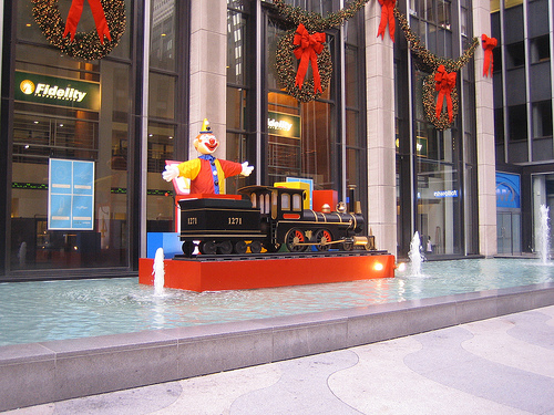
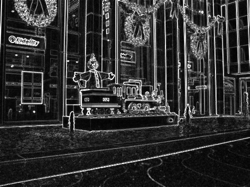
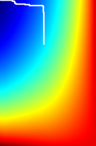
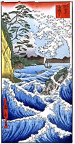
Which is just simply the absolute value of the gradients of the image. In Matlab, I can compute the gradients FX and FY of an image using the built-in method gradients(img), then I just sum the absolute values to compute the energy. Figure 1 is an image and its computed energy function.
|
|
Figure 1: Showcasing the energy of an image.
Let us consider the case where we would like to reduce the width of an image by one. We want to find a vertical seam with the lowest energy and remove it. Recall that a seam is simply an 8-connected path of pixels that is either vertical (top-to-bottom) or horizontal (left-to-right) in an image. The paper proposed a dynamic programming approach for finding the optimal seam in an image (the seam with the lowest energy). Given the energy of an image, one can start from the second row in the image and move row-by-row in a dynamic programming fashion updating a cumulative energy matrix M with the same size as the image. In particular, we compute each (i, j) entry in M as follows:
$$\begin{aligned}
M(i, j) = e(i, j) + \min ( M(i-1, j-1), M(i-1,j), M(i-1, j+1) )\end{aligned}$$
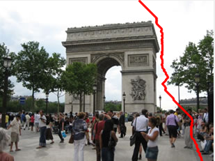
After filling the matrix M, finding the optimal seam is a simple traversal of this matrix starting from the bottom row and moving upwards. The same argument can be made in the case of reducing the height of an image. I coded this process successfully and you can see in Figure 2 the optimal seam colored in red.
|
|
Figure 2: Showcasing the optimal seams of an image highlighted in red.
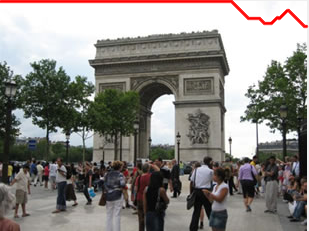
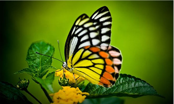
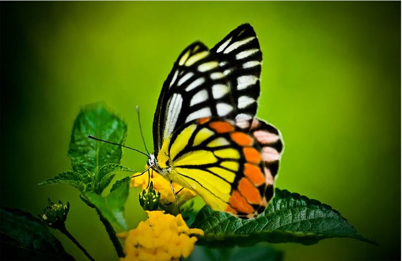
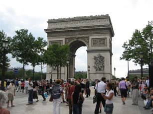
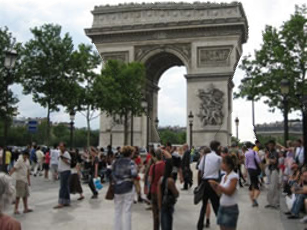
We can successively apply this process again and again to reduce the width of an image to any desired target (the same for reducing the height). Figure 3 showcases the result of reducing the size of an image.
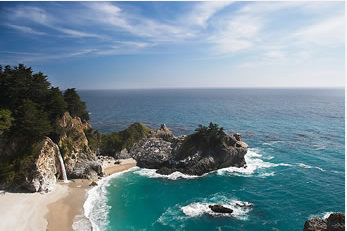
(a) Original image. |
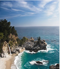
(b) Reducing width by 100 pixels. |
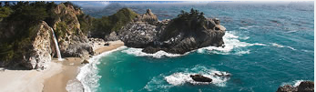
(c) Reducing height of image by 130 pixels. |
Figure 3: Showcasing the use of seam carving to reduce an image. Notice how content is still preserved.
Now consider the case where we would like to reduce the size of an image from n × m to n′×m′. An important aspect of this reduction is in what order should we remove the seams? The paper describes another dynamic programming approach whereby we fill a transport map T. Each entry T(i, j) corresponds to the minimum cost needed to get an image of size n − i × m − j. In particular, the following is the values for each entry:
$$\begin{aligned}
T(i, j) = \min ( T(i-1, j) + e(s^x(I_{n-i-1 \times m-j}), T(i, j-1) + e(s^y(I_{n-i \times m-j-1}) )\end{aligned}$$
Where In − i × m − j is an image of size n − i × m − j and e(s(I)) denotes the energy of the seam that is removed from the image I. Basically, T provides us with a map of the order in which we should remove the seams; if we select the first term then we would remove a vertical seam, whereas the second term corresponds to removing a horizontal seam.
I successfully programmed this component. Figure 4 shows an image and its corresponding transport map and choice path taken for removing the seams.
|
|
|
Figure 4: Result of using the transport map to reduce the size of an image by 90 pixels in both dimensions.
Enlarging an image is a simple process. Consider the case where we would like to increase the width or height by one. First we identify the optimal seam as discussed above (vertical or horizontal). Then we duplicate this seam by averaging it with its left or right neighbors. To increase the size by more than one, we just identify the k optimal seams for removal and duplicate them by averaging. Figure 5] showcases the result of my implementation.
|
|
Figure 5: Result of enlarging an image by 100 pixels in both dimensions.
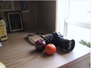
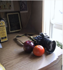
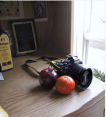
Amplification is the process of enlarging the size of the important contents in an image while maintaining its current dimensions. The paper describes a simple process for doing this: you scale the image by 150%, and then you perform seam carving to reduce the image back to its original dimensions. The result is that unimportant regions in the image will be remove, while important regions will be preserved. Figure 6 showcases the result of my implementation.
|
|
Figure 6: Amplifying the content of an image using scaling and then seam carving..
The paper discussed a problem that can occur when using Seam Carving in the image directly whereby significant artifacts result. To remedy this, they propose using seam carving on the gradient of the image rather than on the image itself. Then once the gradient of the image is reduced to the desired size, we can reconstruct the image using a Poisson solver. I managed to implement this component using a simple Poisson solver Matlab function that I found online 4. Figure 6 showcases the difference between the original method and the gradient domain method for resizing an image. Notice how in the original method, there is are noticeable artifacts.
|
|
|
|
(a) Original image. |
(b) Resized image using normal seam carving. |
(c) Resized image using gradient domain seam carving. |
Figure 7: Showcasing the difference from using gradient domain seam carving. Notice how that there are less artifacts and the image is smoother when using the gradient domain method.
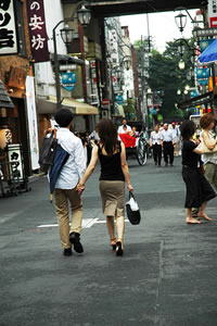
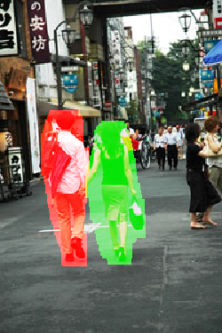
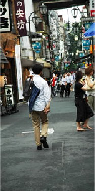
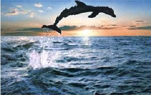
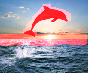
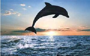
The use of an energy function allows one to create custom metrics for selecting the seams. So, suppose that we’d like to protect a region of an image from being carved, or if we’d like to specify a region for removal. This can easily be done by altering the energy function of those specific regions. Recall that the seam carving algorithm selects the seam with the lowest energy. Thus, in the case of object removal, we just modify the energy of the object pixels to be very low (large negative number). For object protection, we just modify the energy of the object pixels to be very large (large positive number). This way, the algorithm will select/avoid the appropriate seams for the job. Figure 8 showcases the result of seam carving on two regions; green is protected and red is removal.
|
|
|
|
(a) Original image. |
(b) Highlighted regions. |
(c) Resized image with object removed. |
Figure 8: The use of seam carving to protect and remove two regions in an image.
The original seam carving approach of removing the lowest energy seam can cause noticeable artifacts because it disregards the energy that is inserted into an image. This added energy is caused by the creation of edges that were not present in the original image. So to remedy this, in the second paper, the proposed approach selects the seam that inserts the minimum amount of energy into the image. This is called forward energy, whereas the original approach is called backward energy. To implement this via dynamic programming approach, we just need to modify our cost function. For each pixel that we consider for removal, its energy cost will be the difference between its neighbors. Analytically our cumulative energy matrix M now becomes:
$$\begin{aligned}
M(i, j) = \min\begin{cases}
M(i-1, j-1) + |I(i, j+1) - I(i, j-1)| + |I(i-1,j) - I(i,j-1)| \\
M(i-1,j) + |I(i,j+1) - I(i,j-1)|\\
M(i-1, j+1) + |I(i,j+1) - I(i,j-1)| + |I(i-1,j)-I(i,j+1)|
\end{cases}\end{aligned}$$
Since I’ve already implemented the backward energy approach, incorporating forward energy was a straight-forward task. Figure 9 contrasts the difference between applying backward energy and forward energy on an image.

(a) Original image. |
|
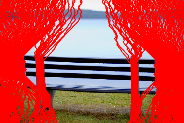
(b) Backward energy seams. |
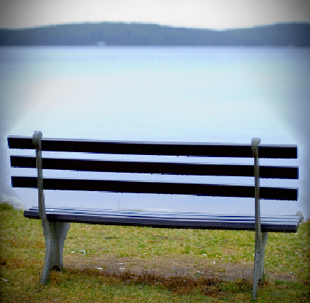
(c) BE Resizing. |
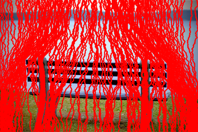
(d) Forward energy seams. |
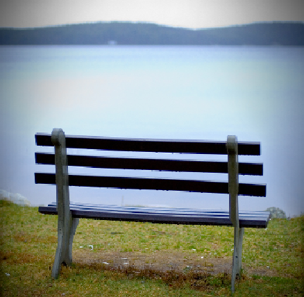
(f) FE Resizing. |
Figure 9: Comparison between backward energy and forward energy. We see that the forward energy result suffers from less artifacts as can be seen by the bench beams and discoloration.
A video consists of multiple frames taken at different timestamps. One naive way to apply seam carving is to simply carve each frame independently of the others, however such an approach can lead to noticeable artifacts and inconsistent frames when playing the video. One simple approach proposed is to compute the energy of each frame, then take the max energy at each pixel, which can be used to identify a seam for carving. Notice that with videos, each pixel location has two energy components: spatial and temporal. The spatial energy can be computed within the same frame, whereas the temporal energy is computed between two consequent frames. If we denote a frame at time t as It, then the temporal energy at pixel (i, j) for the frame It is the gradient of the image with respect to t: |It + 1(i, j)−It(i, j)|.
Having two components for each pixel location allows us to balance the tradeoff between them using a global energy function as follows:
$$\begin{aligned}
E_{spatial}(i,j) = \max_{t=1}^N \{|\frac{\partial}{\partial x}I_t(i,j)| + |\frac{\partial}{\partial y}I_t(i,j)|\}\end{aligned}$$
$$\begin{aligned}
E_{temporal}(i,j) = \max_{t=1}^N \{|\frac{\partial}{\partial t}I_t(i,j)|\}\end{aligned}$$
$$\begin{aligned}
E_{global}(i,j) = \alpha E_{spatial} + (1-\alpha)E_{temporal}\end{aligned}$$
The paper recommends setting α to 0.3 from empirical results. Implementing this was just a matter of computing the energy of each frame and the temporal energy between every two consequent frames. We end up with N spatial energy matrices and N temporal energy matrices for which we take the max for each. Then we sum the two matrices using the global energy formula above. Finally, we apply seam carving using this energy matrix to identify the best seam to carve out of all the frames. Figure 10 shows the result of this video carving approach.
|
|
|
Figure 10: Applying simple video carving using the global energy approach.
To be able to apply seam carving to videos in a more complex manner, we would need a more expressive representation of the frames. In the second paper they proposed a graph cut method for applying seam carving which is equivalent to the dynamic programming approach. This approach can be applied to both images and video. Finding the optimal seam of an image consists of the following steps:
Construct a directed graph representation of the image, i.e. each pixel is a node and adjacent pixels are neighboring nodes.
For the edges, for each pixel, we would add the edges along with their weights according to Figure 11 which illustrates the cases for background and forward energies, respectively.
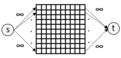
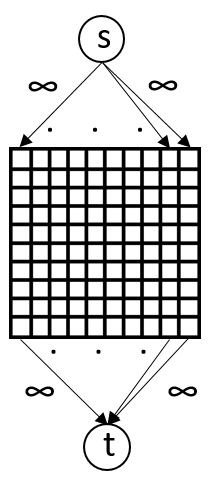
Add a source node s and an edge from s to every pixel in the left-most column with ∞ weight in the case of vertical seams (to every top-most row for horizontal seams). See Figure 12.
Add a sink node t and an edge from every pixel in the right-most column to t with ∞ weight in the case of vertical seams (from every bottom-most row for horizontal seams). See Figure 12.
Apply max-flow/min-cut algorithm which will partition the graph into two disjoint sets S and T. The optimal seam is defined by the minimum cut, in particular we want the pixels whose weights cross from the set S to the set T. Figure 13 illustrates the pixel partitioning into the sets of S and T and the resulting optimal seam for my implementation.

|

|
|
(a) Backward energy graph connections for vertical seam (left) and horizontal seam (right) selection. Here, for the case of vertical seams, $E_1 = | \frac{\partial}{\partial x} I(i,j) | + | \frac{\partial}{\partial y} I(i,j) |$. |
|

|

|
|
(b) Forward energy graph connections for vertical seam (left) and horizontal seam (right) selection. Here, for the case of vertical seams, $+LR = | I(i,j+1) - I(i,j-1) ||$, $+LU = |I(i-1,j) - I(i,j-1) |$, and $-LU = | I(i+1,j) - I(i,j-1)|$. |
|
Figure 11: Illustration of graph connections among pixels.
(a) Vertical seam configuration. |
(b) Horizontal seam configuration. |
Figure 12: Illustration of source $s$ and sink $t$ connections.
|

|

|
|
(a) Original image. |
(b) Vertical seam cut. |
(c) Horizontal seam cut. |
Figure 13: Illustration resulting $S$ (black pixels) and $T$ (white) partitions. The optimal seam pixels are the pixels on the boundary of the $S$ set.
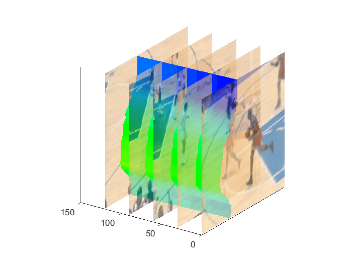
To extend this algorithm to videos, we need to consider adding edges between consequent frames. This can easily be done by adding the edges as shown in Figure 14. For an image, a seam is a 2D object, whereas for videos the seam is 3D surface manifold. Figure 15 illustrates an example of the seam surface that results from my implementation.

|

|
Figure 14: Illustration of temporal graph connections among pixels between consequent frames $t$ and $t+1$. The left image is for vertical seams and right is for horizontal seams.
|
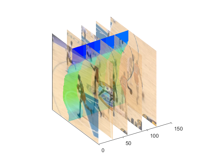
|
Figure 15: Resulting vertical seam manifold using graph cut implementation.
For the implementation details, I used the digraph class in Matlab (introduced in version R2015b) to construct the image/video graphs. Initially, I first constructed an adjacency matrix representation and then passed this as an argument to the digraph class. However, this method suffers from severe memory issues but was fast to construct the graph; an image of size n × m requires a matrix of size n2 × m2, for a video with k requires k2 × n2 × m2. One method that reduces memory limitations is to construct the graph directly by adding the nodes and then the edges one by one. However, this method runs very slowly. To remedy this, I implemented the graph construction in a way that balances between memory and speed, it is faster then the second method but still requires considerable time for large images/videos (1 hour). After constructing the graph, Matlab provides a method called maxflow which takes a digraph object and returns the S and T partitions. The final step is just processing the S set and identifying the pixels that are on the boundary (this can be done by using a binary mask for pixels in S and T).
In the GUI program, if the user loads an image/video file and decides to apply the graph cut implementation, I resize the file to a reasonable size to keep the processing time reasonable. Note that the graph construction is carried for each seam removal operation, i.e. if we remove 8 seams then we perform 8 graph constructions. A more optimized approach would modify the initial graph directly by removing the nodes that are part of the seam and modifying neighboring pixel weights. However, due to deadline constraints and the lack of foresight in designing the framework for my code I could not complete this optimized approach. Figure 16 showcases the graph cut method applied to a video file.
|
|
|
Figure 16: Applying graph cut seam carving to enlarge video.
I implemented a simple GUI program in Matlab that includes all the components discussed so far. A user can load an image/video and reduce or enlarge an image/video to a desired target. The program also enables a user to see the seams that are selected by a resizing operation. The user can also amplify an image as discussed above. There is also the ability to highlight parts of an image for protection and removal. Finally, when applying graph cuts, the program will resize the image/video to a reasonable size due to the time limitations of this method. Figure 17 shows the current program interface and its functionality.
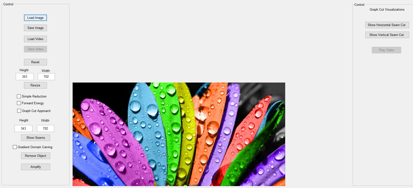
|
Figure 17: The interface of the current GUI program that I have developed.
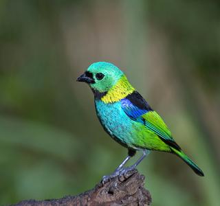
Let’s compare seam carving to two known approaches for reducing the size of an image: scaling and cropping. Figure 18 shows an image and the resulting reduced images using: scaling, cropping, backward energy, and forward energy. We would like to preserve the main contents of an image, and we see that scaling does not achieve this as it just uniformly reduces the size of all objects. Whereas, seam carving achieves results that are very similar to cropping. Furthermore, we see how forward energy reduces the resulting artifacts as can be seen by comparing the tail of the bird between the backward and forward energy results.
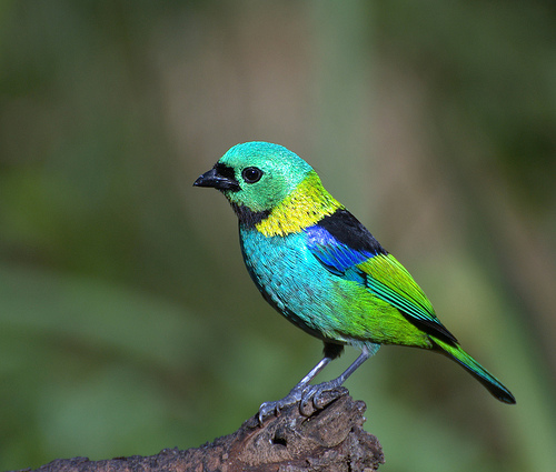
(a) Original image. |
(b) Scaled image. |
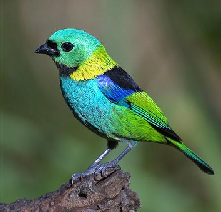
(c) Cropped image. |
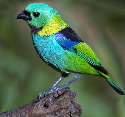
(d) BE seam carving. |
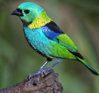
(e) FE seam carving. |
Figure 18: Comparison between scaling and seam carving. Notice how forward energy seam carving achieves results similar to cropping.
The main limitation of seam carving is that it cannot be applied automatically to all images, we would need to aid it by either incorporate object detection or user aid to highlight the important content in an image so that it is not carved. Figure 19 showcases an example where seam carving an image fails, but if we highlight important parts in the image, it produces good results.
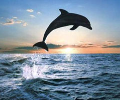
|
|
|
|
Figure 19: The effects of using object detection to aid seam carving in achieving good results.
There are also situations in which even object detection with seam carving will not work. If there is a lot of content in an image, then any content retargeting technique will be severely impacted. Figure 20 showcases this situation.
(a) Original image. |
(b) Seam carved image. |
Figure 20: Too much content results in bad seam carved images.
In this project we have implemented and shown the results of using seam carving on images/videos. With the use of aided object detection seam carving can achieve very good results. Furthermore, to decrease the processing time required, one can pre-compute the index maps for the seam removal operations beforehand and then carve to the required size in real-time (this was not implemented in this project). Seam carving is severely influenced by the energy function that is used, a look into more robust energy measures can help in attaining better results. For video, one can apply object recognition and motion to help maintain important content while using seam carving. Finally, I’d like to say that all the code accompanied has been implemented by me using standard Matlab functions except in the case of the poisson solver which I have obtained at [4], the digraph for computing the minimum cuts, the gradient method for computing the gradients, and the regionprops method for getting mask information.
I’d also like to acknowledge the images/videos that I have obtained from here, the seam carving creator’s website. The bear video can be found at: here.
[1] Avidan S., Shamir A. Seam carving for content-aware image resizing (2007). http://www.faculty.idc.ac.il/arik/SCWeb/imret/imret.pdf
[2] Rubinstein M., Avidan S., Shamir A. Improved Seam Carving for Video Retargeting (2008). http://www.faculty.idc.ac.il/Arik/SCWeb/vidret/vidret.pdf
[3] Rubinstein M., Gutierrez D., Sorkine O., Shamir A. A Comparative Study of Image Retargeting. (2010). http://people.csail.mit.edu/mrub/papers/retBenchmark.pdf
[4] Agrawal A. Graph Cuts, Bilateral filtering and Gradient domain reconstruction. http://web.media.mit.edu/raskar/photo/code.pdf