The XOR dataset consists of the following two point sets in 2-dimensional Euclidean space: A = { (0,0), (1,1) }, B = { (1,0), (0,1) }. The two sets A and B are represented in the MATLAB environment as the two matrices A and B. The matrix A is entered into the MATLAB environment by typing, at the MATLAB prompt (>>):
>> A = [ 0 0; 1 1 ]
Similarly, the matrix B is entered as follows:
>> B = [ 1 0 ; 0 1 ]
The decision tree that separates the sets A and B is generated as follows (the decision tree will be represented in the MATLAB environment as the matrix T):
>> T = msmt_tree(A,B)
The decision tree separating the sets A and B is represented by the following matrix T:
T =
	2	-2
       -2	 2
	1	 1
	2	-1
       -1	-1
	1	 2
Only "decision nodes", nodes indicating an error-minimizing separating plane in the tree, are represented in the matrix T. Each column of T contains the following information: the linear coefficient w and the translation theta of the error-minimizing separating plane wx = theta, the index of the left child of the current decision node, the index of the right child of the current decision node, and information needed to display the tree (see Example of Displaying Decision Tree Generated with XOR Dataset).
For a given column in the matrix T (equivalently, decision node in the tree), the linear coefficient w is represented as the first n entries in the column. The translation theta is represented as the n+1 entry in the column. The n+2 entry in the column is the index to the node representing the left child of this decision node. The left child node then separates all points x such that wx <= theta. If the n+2 entry is -1, this indicates that the left child of this decision node is a leaf node (i.e. all points x such that wx <= theta are elements of set A ). The n+3 entry in the column is the index to the node representing the right child of this decision node. The right child then separates all points x such that wx > theta. If the n+3 entry is -1, this indicates that the right child of this decision node is a leaf node (i.e. all points x such that wx > theta are elements of the set B ).
Thus, for the matrix T representing the decision tree describing the separation of the XOR problem:
T =
	2	-2
       -2	 2
	1	 1
	2	-1
       -1	-1
	1	 2
The first column indicates that the first error-minimizing separating plane is given by w_1 = [ 2 -2 ], theta_1 = 1, the left child of this decision node is in column 2, the right child of this decision node is a leaf node (indicating that any point x of the XOR problem such that (w_1)x > theta_1 belongs to the set B ). The second column represents the error-minimizing separating plane needed to separate all the points x of the XOR problem such that (w_1)x <= theta_1. This error-minimizing plane is given by w_2 = [ -2 2 ], theta_2 = 1, the left child of this decision node is a leaf node (indicating that any point x of the XOR problem such that (w_1)x <= theta_1 and (w_2)x <= theta_2 belongs to the set A ), and the right child of this decision node is a leaf node (indicating that any point x of the XOR problem such that (w_1)x <= theta_1 and (w_2)x > theta_2 belongs to the set B ).
For further information regarding the semantics to the columns of T, and the generation of decision tree, see msmt_tree.m file.
See Example of Decision Tree Generation with XOR Dataset for information regarding the generation of the decision tree.
We assume that in the MATLAB environment, the decision tree is represented as the matrix T, and the sets A and B of the XOR dataset are represented as the matrices A and B. The decision tree is then displayed by entering the following command at the MATLAB prompt (>>):
>> disp_tree(T,A,B)
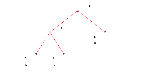
MATLAB produces the following graphical representation of the decision tree:
Each node of the tree is numbered. The following information is displayed corresponding to each numbered node in the graphical representation of the decision tree:
Plane:  wx = theta

Node #     w                 theta     # Pts. of A  # Pt. of B

1        2.000  -2.000       1.000         2            2

2       -2.000   2.000       1.000         2            1

3       Leaf Node                          2            0

4       Leaf Node                          0            1

5       Leaf Node                          0            1
See disp_tree.m file.
The Wisconsin Breast Cancer Dataset consists of two point sets in 9-dimensional Euclidean space: B and M . B is made up of 444 points representing measurements from 444 tumors known to be benign. M is made up of 239 points representing measurements from 239 tumors known to be malignant. These sets are represented in the MATLAB environment as the 444 x 9 matrix B and the 239 x 9 matrix M.
See Example of Decision Tree Generation with XOR Dataset for information regarding the generation of the decision tree to separate the sets B and M .
We assume that in the MATLAB environment, the decision tree is represented as the matrix T, and the sets B and M of the Wisconsin Breast Cancer Dataset are represented as the matrices B and M.
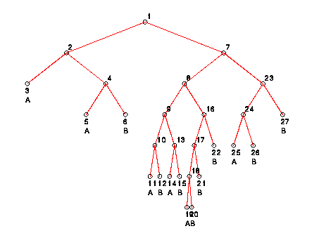
The following is the graphical representation of the full decision
tree constructed to separate the sets B
and M in 9-dimensional Euclidean space:
It is possible to prune this decision tree in 2 ways: (1) using the pruning algorithm proposed by Quinlan in C4.5: Programs for Machine Learning, and (2) by a minimum-point algorithm.
The pruning algorithm proposed by Quinlan requires that at "certainty factor" (CF) be provided. The value of the "certainty factor" is in the range 0 <= CF <= 1.0. For a detailed description of this pruning algorithm, see:
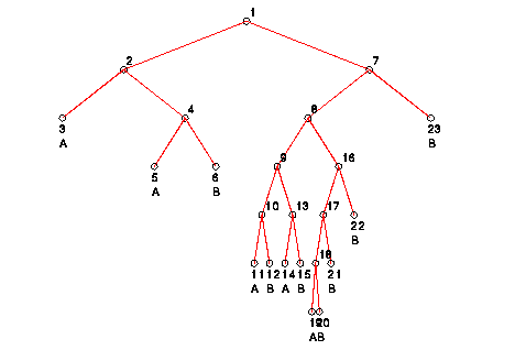
The original decision tree can be "pruned" using the following command (CF = 0.25, the resulting "pruned tree is stored as matrix TT):
>> TT = prune_tree_C45(T,B,M,0.25)
The following is a graphical representation of the "pruned" tree
(notice that leaf nodes 24, 25, 26, and 27 have been "pruned"):
See prune_tree_C45.m file.
Similarly, the original tree can be pruned by a Minimum Points pruning algorithm. This algorithm requires that a "minimum number of points" (min_points) parameter be provided. The original tree is then pruned as follows: if any node of the decision tree misclassifies less than min_points points, then the node is changed into a leaf node.
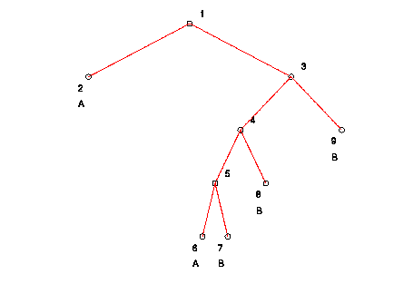
The original decision tree can be "pruned" using the following command (min_points = 10, the resulting "pruned" decision tree will be represented by the matrix TTT):
>> TTT = prune_tree_points(T,B,M,10)
The following is a graphical representation of the "pruned" tree
(notice that many of the nodes have been pruned):
See prune_tree_points.m file.
Cross validation is used to test how well a given decision tree will correctly classify data that has not been presented (generalize). For more information regarding cross validation, please see:
10-fold cross validation can be performed using the Wisconsin Breast Cancer Dataset using the following command:
>> [percent,C,ave_planes,stdev] = cross_val(B,M,10)
For each fold of the 10-fold cross-validation, the following information is provided: total number of points in the testing set correctly classified, total number of points in the testing set incorrectly classified, the percentage of points in the testing set correctly classified. When cross-validation has finished, "percent" is the average percentage of points (testing set) correctly classified, "C" is a confusion matrix, "ave_planes" is the average number of separating planes needed, "stdev" is the standard deviation in percentage of points of testing set correctly classified for each fold.
For the Wisconsin Breast Cancer Dataset, the results produced are:
Count  Total Correct  Total Incorrect  Percentage Correct

1        63.000         5.000           92.647
2        63.000         6.000           91.304
3        66.000         2.000           97.059
4        66.000         3.000           95.652
5        64.000         4.000           94.118
6        65.000         2.000           97.015
7        62.000         7.000           89.855
8        63.000         5.000           92.647
9        67.000         2.000           97.101
10        65.000         3.000           95.588

percent =

   94.2899

C =

   429    24
    15   215


ave_planes =

   10.8000


stdev =

    2.5937