Russell Manning > Research > Fast Self Calibration
Our initial publication concerning screw-transform
manifolds included a simple algorithm for performing self calibration
(click here for a discussion of self
calibration and screw-transform manifolds). This was a voting
algorithm and amounted to a Hough transformation for self
calibration. The algorithm had the strengths and weaknesses of any
Hough-like algorithm: it was robust to outliers but was slow and
required large amounts of memory. Furthermore, the results of the
voting process could be ambiguous.
Recently, we developed a fast alternative to the
voting algorithm that makes self calibration from screw-transform
manifolds not just feasible but possibly the premier method for self
calibration. This work is currently under review for publication so we
can not discuss the details of the method here. However, some of our
results are discussed below.
Here are the strengths of our algorithm:
operates quickly
and reliably
works from the theoretical minimum
of 3 camera views
can be used
efficiently with RANSAC for robustness
determines all
possible self calibrations in a single pass
makes normalization
of the calibration search space possible
|
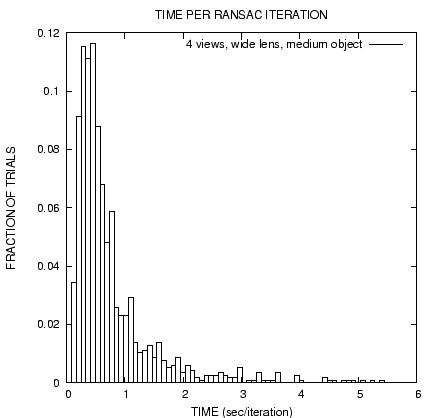
Speed
The speed of our algorithm is demonstrated by the histogram on the
left. Several hundred trials on noisy, synthetic data were run;
each trial consisted of several RANSAC iterations and each
iteration involved 3 fundamental matrices. These experiments were
run on a Sun UltraSparc. The histogram shows the distribution of
runtimes for each RANSAC iteration; the vast majority of
iterations took under 1 second.
|
|
|
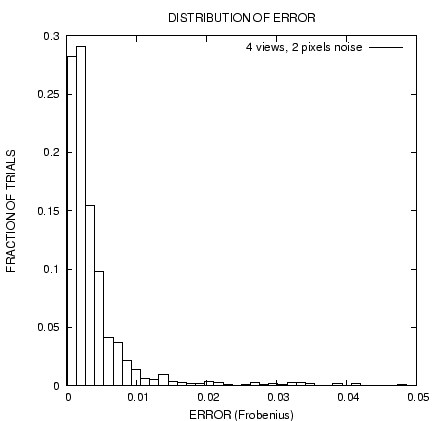
Accuracy
The histogram on the right shows the distribution of calibration
error for several hundred trials on synthetic data. The synthetic
images were 1000x1000 pixels in size and uniform noise with a
radius of 2 pixels in both the x and y direction was added to the
feature points; there were about 100 feature points, and the
standard deviation of the features on each camera's image plane
was about 170 pixels (this is a measure of the retinal size of the
object; the object covered 1/3 to ½ of each camera's view).
As a general rule, near-perfect reconstructions are achieved when
Frobenious error is below 0.001.
|
|
|
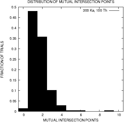
Possible
Calibrations
It is unknown how many possible internal calibration matrices are
consistent with a given triplet of views in general configuration.
An upper bound of 21 was given by Shaffalitzky. Our method makes
it possible to estimate this number experimentally. The histogram
on the right shows the number of legal internal calibration
matrices found for a randomly generated triplet of camera views;
several hundred trials were performed, each with a different
randomly-generated triplet, and the results are shown as a
distribution. These results suggest that only 1 or 2 calibrations
are possible for 3 camera views in general configuration.
|
|
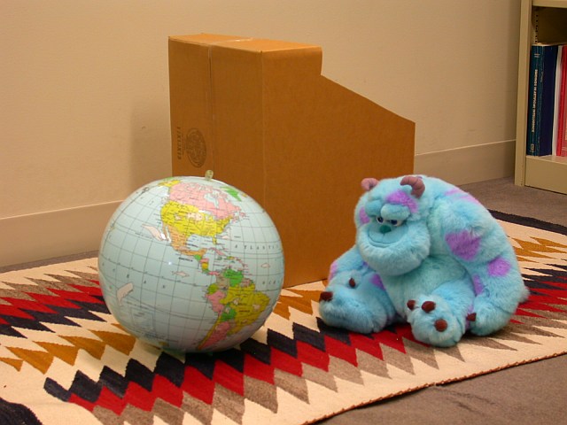
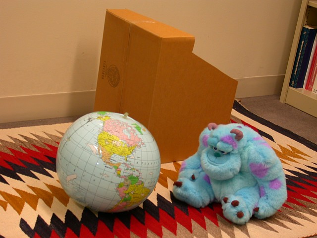
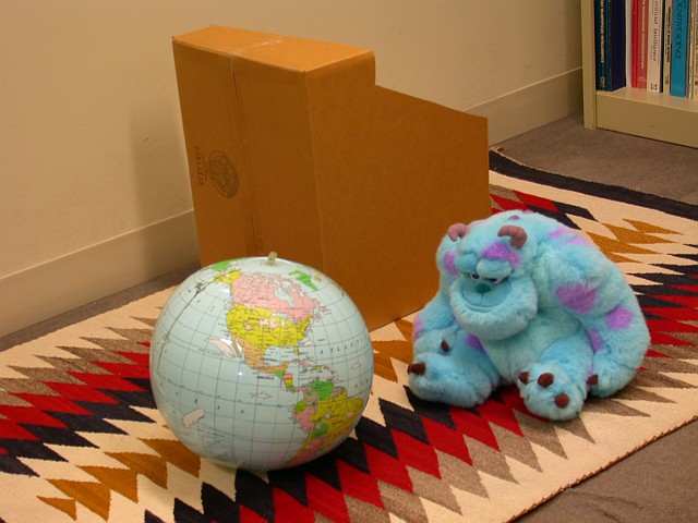
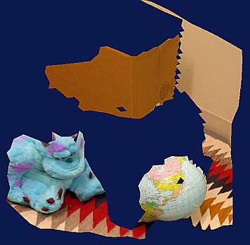
Here is an example of self calibration and scene reconstruction
from real photographs. Fig. 1 shows the 3 original camera views used
in the process; each view was taken by the same camera (from different
positions) without changing the camera's internal parameters. Note
that the views are fairly closely positioned in space and that the
camera introduced some radial lens distortion, which was not corrected
for. The calibration process was more difficult due to these last two
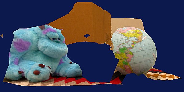
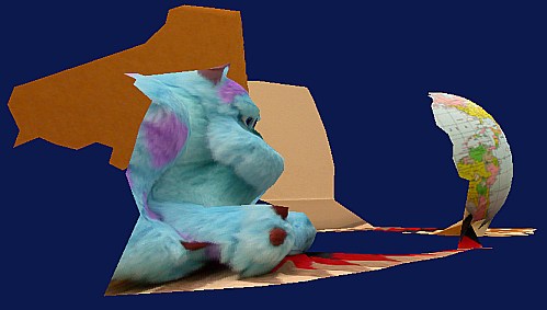
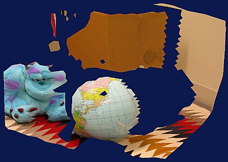
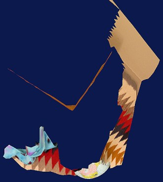
observations. Fig. 2 shows several views of the reconstructed scene;
the reconstruction is mirror reversed. Note in the last (overhead)
view that the two walls of the box are at right angles.
A movie of the reconstruction is available as an ".avi" file; use
the DivX version if possible:
[0.65M (DivX codec)]
[2.2M (Indeo codec)]
A longer movie of the reconstruction; this version runs in a closed loop:
[2.8M (DivX codec)]
[9.4M (Indeo codec)]
|
Fig.
1: Original Camera Views
|
|
|
|
|
|
Fig.
2: Scene Reconstructions
|
|
|
|
|
|
|
|
|
|
|
|
Russell Manning / rmanning@cs.wisc.edu / created 01/27/03 / last modified 02/15/03
|