Understanding Variance Reduction Techniques with SGD

Stochastic Gradient Descent (SGD) is the workhorse behind many machine learning tasks. It’s used to train many common classifiers like linear classifiers and SVMs, as well as large non-convex problems like neural networks. In general, SGD has a small memory footprint, learns quickly, and is robust to noise- all good things to have in a training algorithm. However, SGD has high variance between applications of the gradient function which can be inefficient. The research community has addressed this problem by introducing Variance Reduction (VR) techniques.

In this article, we wish to give an intuitive understanding of how variance reduction (VR) techniques work when applied to SGD. To this end, we have constructed an interactive visualization of an SVM learning in real time, using one of 3 possible update algorithms. We also implemented several algorithms in C++ and tested them on real world datasets to learn how the algorithm’s differ in time to convergence.

SGD Background

In its simplest form, we can write the stochastic update function as

$$w_{i+1} = w_{i} - \eta(\nabla f_i(x_j))$$

where $x_j$ is single randomly selected training example, and $w_i$ is the weight vector at time $i$. $\nabla f$ is the gradient of our loss function, $f$. Each iteration $i$ changes the weight vector by taking a step of size $\eta$ in the opposite direction of greatest positive change (i.e. we are reducing the loss). After some number of iterations, or when $w_{i} - w_{i+1}$ is sufficiently small, we consider ourselves converged.

SGD is often compared to the Gradient Descent which, instead of calculating $\nabla f_i(x_j)$, calculates $\nabla f_i(X)$ where $X$ is the entire training set. $\nabla f_i(X)$ is sometimes called the true gradient because it is the actual gradient at $i$ whereas $\nabla f_i(x_j)$ is merely an approximation of the true gradient at $i$. Because gradients in GD are accurate, we can use a larger learning rate than SGD. However, SGD generally converges faster than GD. If $n$ is the number of training examples, we generally use let $\eta _{SGD} > \frac{\eta _{GD}}{n}$ meaning that if SGD’s gradients are mostly accurate, we should converge faster than GD because we apply many more gradient per unit time.

One of the main weaknesses of SGD is the imprecision of the stochastic gradients. The problem is that gradients tend to bounce around in varying directions, so instead of smoothly approaching our converged error, we will tend to jitter.

The image shows a sketch of the error rate as we train. In the ideal case, error should be strictly decreasing, however, this is often not the case for SGD.

VR Algorithms Overview

ASGD

Averaged Stochastic Gradient Descent is the simplest method of variance reduction. We use the formulation given by Leon Bottou in [1]. The VR stochastic update works by keeping an average of some set of the weight vectors, and using this average as the true weight vector. We’ll define the average as

$$\bar{w}_t = \frac{1}{t - t_0}\sum_{i=t_0}^{t}w_i$$

This means that we will need to select a $t_0$. There’s no clear guideline on how to do this, so in our experiments and in our visualization, we choose to begin averaging after the first epoch. For each update before $t_0$, we do a normal stochastic update:

$$w_{t+1} = w_{t} - \eta(\nabla f_t(x_j))$$

Then, we swap out the stochastic weight vector with an averaged one, given as:

$$\bar{w}_{t+1} = \bar{w_t} + \mu_t (\bar{w_t} - w_t)$$

where $\mu_t$ is $\frac{1}{max(t-t_0, 1)}$. The max is needed in case we start $t_0$ at time zero.

Notice, we still compute the stochastic gradient at each iteration, but we keep a running average the gradient since $t$.

It’s easy to see how variance is reduced using this method, as now we take only small differences from the average and the newly computed gradient. That, and since we choose time $t_0$ to be large, we should already be close to converging, so changes will be minimal anyways.

SAG

SAG, Stochastic Averaged Gradient, builds on the ASGD method by keeping a history of $n$ past gradients, as well as the moving average of the last epoch’s worth of updates. The method is described thoroughly in [2].

The update function is given as:

$$w_{t+1} = w_{t} - \eta\left[\frac{f'_t(w_t)-f'_{\hat{t}}(\phi_{\hat{t}})}{n} + \frac{1}{n}\sum_{i=1}^{n}f'_i(\phi_i)\right]$$

It’s worth noting that the authors go into various modifications of the original algorithm which improve over the basic update as given above.

SAGA

SAGA has a very similar update function.

$$w_{t+1} = w_{t} - \eta\left[{f'_t(w_t)-f'_{\hat{t}}(\phi_{\hat{t}})} + \frac{1}{n}\sum_{i=1}^{n}f'_i(\phi_i)\right]$$

The original paper does an excellent job of comparing several VR methods [3].

Note that we say $\hat{t}$ as the previous iteration’s corresponding value for the weight vector.

SVRG

SVRG, Stochastic Variance Reduced Gradient, is the final method which we are looking at. It’s update function is given as:

$$w_{t+1} = w_{t} - \eta\left[{f'_t(w_t)-f'_{\hat{t}}(\tilde{w})} + \frac{1}{n}\sum_{i=1}^{n}f'_i(\tilde{w})\right]$$

The original paper describing the algorithm can be found here [4].

How they compare

All three algorithms in SAG, SAGA, SVRG require that an entire epoch’s worth of gradients be stored. This can be very cheap in the case of logistic or linear regression as we only need to save a single variable as the gradient. In most models, however, we increase our memory requirement by the size of the training data.

ASGD has the lowest memory footprint, and is the easiest to implement.

Visualizing Variance Reduction Methods

To gain an intuitive understanding of how gradient descent methods converge to a solution, we created a visualization of an SVM learning to seperate 2 dimensional data.

You can select the solver algorithm, the hyper-parameters of the solvers. You may find that decreasing the learning rate is necessary for the solver to give a stable solution.

Our data is randomly generated using a guassian distribution centered at an equal distance from the origin. You can change the mean of the distribution to see how solvers handle data which is and is not seperable.

A description of each solver is below the visualization.

The number labeled i in the corner of the visualization is the iteration over the data set: for each example processed, i is incremented.

The number labeled e is the epoch, or how many times the complete data set has been parsed over.

The lambda parameter changes how much the SVM will punish misclassified examples. Another way of saying this is that decreasing lambda should decrease the margin.

Performance Comparison

In order to evaluate the success of the different SGD solvers, we implemented them as they are explained in the literature. Then, we analyzed their performance on commonly used LIBSVM datasets which can be found on this page.

We implemented these algorithms in C++ using the Eigen library, which allowed us to run linear algebra operations on large datasets with high speed.

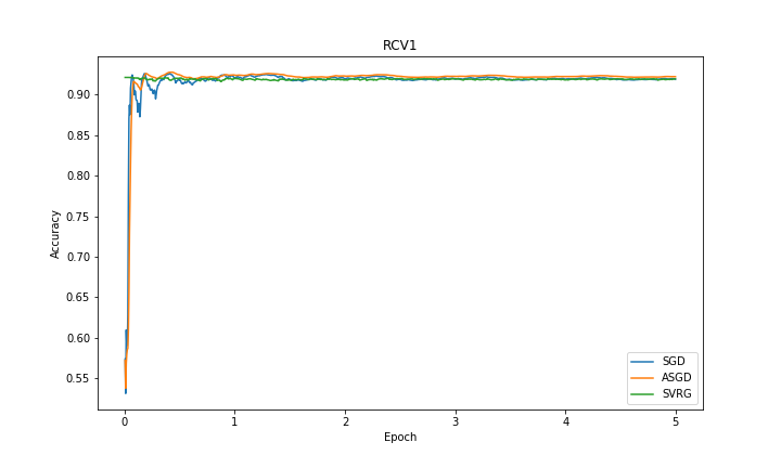
As for the datasets, we used the RCV1 and EPSILON datasets. RCV1 is used for research on text categorization and has 47,236 features. It contains 20,242 and 677,399 examples respectively in the training and test dataset. EPSILON was used in PASCAL Challenge 2008 and has 2,000 features. It contains 400,000 and 100,000 examples respectively in the training and test dataset. Both datasets are for binary classification problems.

We ran our experiments on Macbook Pro 2017 with 4-Core 2.9 GHz Intel i7 Skylake CPU and 16 GB 2133 MHz LPDDR3 memory.

Note you can click on the pictures to enlarge them.

Dataset	Error	Accuracy
RCV1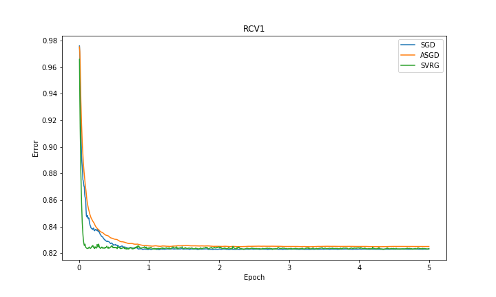
EPSILON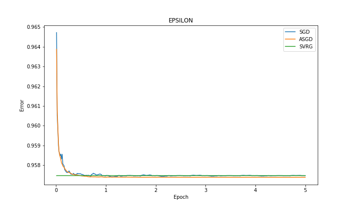

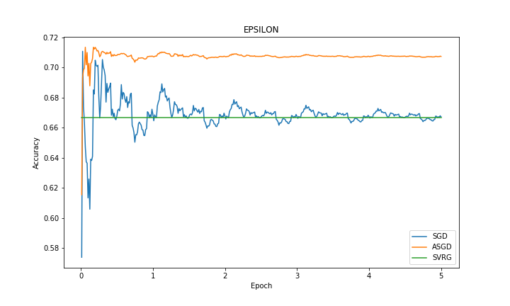Link to Repository

Findings

In experiments, we observed that SVRG is faster than other methods to converge to optimal error rate in both datasets. The accuracy of the methods in RCV1 dataset are close to each other whereas ASGD’s accuracy is better than the rest in EPSILON dataset. We omitted the results from SAG and SAGA because we observed fluctuations of performance in both RCV1 and EPSILON dataset. Our reasoning was that there was a numerical problem in the way that we did our calculations.

Works Cited

1. [1]Bottou, L. 2012. Stochastic Gradient Descent Tricks. Neural Networks: Tricks of the Trade: Second Edition. G. Montavon et al., eds. Springer Berlin Heidelberg. 421–436.
2. [2]Schmidt, M. et al. 2013. Minimizing Finite Sums with the Stochastic Average Gradient. CoRR. abs/1307.2388, (2013).
3. [3]Defazio, A. et al. 2014. SAGA: A Fast Incremental Gradient Method With Support for Non-Strongly Convex Composite Objectives. CoRR. abs/1407.0202, (2014).
4. [4]Johnson, R. and Zhang, T. 2013. Accelerating Stochastic Gradient Descent Using Predictive Variance Reduction. Proceedings of the 26th International Conference on Neural Information Processing Systems (USA, 2013), 315–323.