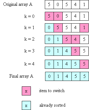
Selection Sort
The idea behind selection sort is:
- Find the smallest value in A; put it in A[0].
- Find the second smallest value in A; put it in A[1].
- etc.
- Use an outer loop from 0 to N-1 (the loop index, k, tells which position in A to fill next).
- Each time around, use a nested loop (from k+1 to N-1) to find the smallest value (and its index) in the unsorted part of the array.
- Swap that value with A[k].
Here's the code for selection sort:
public static void selectionSort(Comparable[] A) {
  int j, k, minIndex;
  Comparable min;
  int N = A.length;

  for (k = 0; k < N; k++) {
     min = A[k];
     minIndex = k;
     for (j = k+1; j < N; j++) {
        if (A[j].compareTo(min) < 0) {
	    min = A[j];
	    minIndex = j;
	}
     }
     A[minIndex] = A[k];
     A[k] = min;
  }
}
And here's a picture illustrating how selection sort works:
What is the time complexity of selection sort? Note that the inner loop executes a different number of times each time around the outer loop, so we can't just multiply N * (time for inner loop). However, we can notice that:
- 1st iteration of outer loop: inner executes N - 1 times
- 2nd iteration of outer loop: inner executes N - 2 times
- ...
- Nth iteration of outer loop: inner executes 0 times
-
N-1 + N-2 + ... + 3 + 2 + 1 + 0
What if the array is already sorted when selection sort is called? It is still O(N2); the two loops still execute the same number of times, regardless of whether the array is sorted or not.
It is not necessary for the outer loop to go all the way from 0 to N-1. Describe a small change to the code that avoids a small amount of unnecessary work.
Where else might unnecessary work be done using the current code? (Hint: think about what happens when the array is already sorted initially.) How could the code be changed to avoid that unnecessary work? Is it a good idea to make that change?
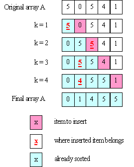
The idea behind insertion sort is:
Here's the code:
Here's a picture illustrating how insertion sort works on the same array
used above for selection sort:
What is the time complexity of insertion sort?
Again, the inner loop can execute a different number of times for every
iteration of the outer loop. In the worst case:
As mentioned above, merge sort takes time O(N log N), which is quite a
bit better than the two O(N2) sorts described above (for example,
when N=1,000,000, N2=1,000,000,000,000, and N log2 N
= 20,000,000;
i.e., N2 is 50,000 times larger than N log N!).
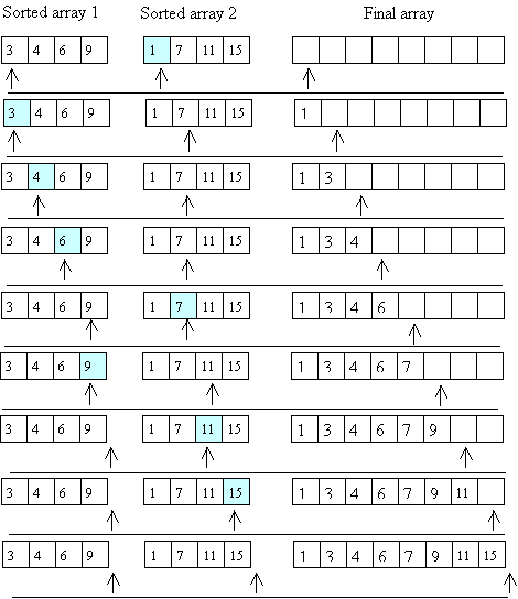
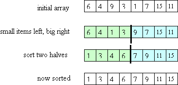
The key insight behind merge sort is that it is possible to
merge two sorted arrays, each containing N/2 items to form one
sorted array containing N items in time O(N).
To do this merge, you just step through the two arrays, always choosing
the smaller of the two values to put into the final array (and only advancing
in the array from which you took the smaller value).
Here's a picture illustrating this merge process:
Now the question is, how do we get the two sorted arrays of size N/2?
The answer is to use recursion; to sort an array of length N:
An outline of the code for merge sort is given below.
It uses an auxiliary method with extra parameters that tell what part
of array A each recursive call is responsible for sorting.
Fill in the missing code in the mergeSort method.
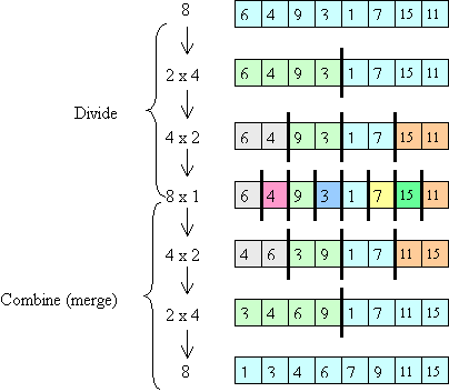
Algorithms like merge sort -- that work by dividing the problem in
two, solving the smaller versions, and then combining the solutions --
are called divide and conquer algorithms.
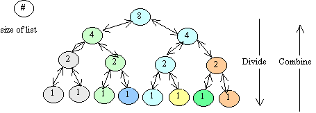
Below is a picture illustrating the divide-and-conquer aspect of merge sort
using a new example array.
The picture shows the problem being divided up into smaller and smaller
pieces (first an array of size 8, then two halves each of size 4, etc).
Then it shows the "combine" steps: the solved problems of half size
are merged to form solutions to the larger problem.
(Note that the picture illustrates the conceptual ideas -- in an actual
execution, the small problems would be solved one after the other, not
in parallel.
Also, the picture doesn't illustrate the use of auxiliary arrays during the
merge steps.)
To determine the time for merge sort, it is helpful to visualize the calls
made to mergeAux as shown below (each node represents
one call, and is labeled with the size of the array to be sorted by that call):
The height of this tree is O(log N).
The total work done at each "level" of the tree (i.e., the work done by
mergeAux excluding the recursive calls) is O(N):
What happens when the array is already sorted (what is the running time
for merge sort in that case)?
Quick sort (like merge sort) is a divide and conquer algorithm:
it works by creating two problems of half size, solving them recursively,
then combining the solutions to the small problems to get a solution
to the original problem.
However, quick sort does more work than merge sort in the "divide" part,
and is thus able to avoid doing any work at all in the "combine" part!
The idea is to start by partitioning the array: putting all small
values in the left half and putting all large values in the right half.
Then the two halves are (recursively) sorted.
Once that's done, there's no need for a "combine" step: the whole array
will be sorted!
Here's a picture that illustrates these ideas:
The key question is how to do the partitioning?
Ideally, we'd like to put exactly half of the values in the left
part of the array, and the other half in the right part;
i.e., we'd like to put all values less than the median value
in the left and all values greater than the median value in the right.
However, that requires first computing the median value (which is too
expensive).
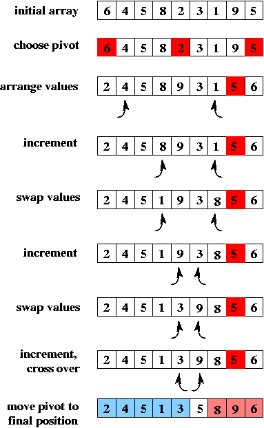
Instead, we pick one value to be the pivot, and we put all values
less than the pivot to its left, and all values greater than the pivot
to its right (the pivot itself is then in its final place).
Here's the algorithm outline:
Now let's consider how to choose the pivot item.
(Our goal is to choose it so that the "left part" and "right part"
of the array have about the same number of items -- otherwise we'll get
a bad runtime).
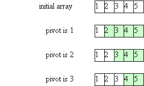
An easy thing to do is to use the first value -- A[low] -- as the pivot.
However, if A is already sorted this will lead to the worst possible runtime,
as illustrated below:
In this case, after partitioning, the left part of the array is empty, and
the right part contains all values except the pivot.
This will cause O(N) recursive calls to be made (to sort
from 0 to N-1, then from 1 to N-1, then from 2 to N-1, etc).
Therefore, the total time will be O(N2).
Another option is to use a random-number generator to choose a random
item as the pivot.
This is OK if you have a good, fast random-number generator.
A simple and effective technique is the "median-of-three": choose the
median of the values in A[low], A[high], and A[(low+high)/2].
Note that this requires that there be at least 3 items in the array, which is
consistent with the note above about using insertion sort when the piece
of the array to be sorted gets small.
Once we've chosen the pivot, we need to do the partitioning.
(The following assumes that the size of the piece of the array
to be sorted is greater than 3.)
The basic idea is to use two "pointers" (indexes) left and right.
They start at opposite ends of the array and move toward each other
until left "points" to an item that is greater than the pivot (so it
doesn't belong in the left part of the array) and right "points" to
an item that is smaller than the pivot. Those two "out-of-place" items
are swapped, and we repeat this process until left and right cross:
Note: If the array may contain a lot of duplicate values, then
it is important to handle copies of the pivot value efficiently.
In particular, it is not a good idea to put all values strictly less
than the pivot into the left part of the array, and all values greater
than or equal to the pivot into the right part of the array. The code
given above for partitioning handles duplicates correctly.
Here's a picture illustrating quick sort:
What is the time for Quick Sort?
What happens when the array is already sorted (what is the running time
for quick sort in that case, assuming that the "median-of-three" method
is used to choose the pivot)?
Insertion Sort
As for selection sort, a nested loop is used;
however, a different invariant holds: after the ith time around the outer loop,
the items in A[0] through A[i-1] are in order relative to each other (but are
not necessarily in their final places).
Also, note that in order to insert an item into its place in the (relatively)
sorted part of the array, it is necessary to move some values to the right
to make room.
public static void insertionSort(Comparable[] A) {
  int k, j;
  Comparable tmp;
  int N = A.length;

  for (k = 1; k < N, k++) {
     tmp = A[k];
     j = k - 1;
     while ((j > = 0) && (A[j].compareTo(tmp) > 0)) {
         A[j+1] = A[j]; // move one value over one place to the right
         j--;
     }
     A[j + 1] = tmp; // insert kth value in correct place relative to previous
                     // values
  }
}
So we get:
1 + 2 + ... + N-1
which is still O(N2).
Merge Sort
The base case for the recursion is when the array to be sorted is of
length 1 -- then it is already sorted, so there is nothing to do.
Note that the merge step (step 4) needs to use an auxiliary array (to avoid
overwriting its values).
The sorted values are then copied back from the auxiliary array to the
original array.
public static void mergeSort(Comparable[] A) {
  mergeAux(A, 0, A.length - 1); // call the aux. function to do all the work
}

private static void mergeAux(Comparable[] A, int low, int high)
{
  // base case
     if (low == high) return;

  // recursive case
  // Step 1: Find the middle of the array (conceptually, divide it in half)
     int mid = (low + high) / 2;
  // Steps 2 and 3: Sort the 2 halves of A
     mergeAux(A, low, mid);
     mergeAux(A, mid+1, high);

  // Step 4: Merge sorted halves into an auxiliary array
     Comparable[] tmp = new Comparable[high-low+1];
     int left = low;    // index into left half
     int right = mid+1; // index into right half
     int pos = 0;       // index into tmp

     while ((left <= mid) && (right <= high)) {
	// choose the smaller of the two values "pointed to" by left, right
	// copy that value into tmp[pos]
	// increment either left or right as appropriate
	// increment pos
	...
     }
     // here when one of the two sorted halves has "run out" of values, but
     // there are still some in the other half; copy all the remaining values
     // to tmp
     // Note: only 1 of the next 2 loops will actually execute
       while (left <= mid) { ... }
       while (right <= high) { ... }

     // all values are in tmp; copy them back into A
       arraycopy(tmp, 0, A, low, tmp.length);
}
Therefore, the time for merge sort involves
O(N) work done at each "level" of the tree that represents the recursive calls.
Since there are O(log N) levels, the total worst-case time is O(N log N).
Quick Sort
Note that, as for merge sort, we need an auxiliary method with two extra
parameters -- low and high indexes to indicate which part of the array to
sort.
Also, although we could "recurse" all the way down to a single item,
in practice, it is better to switch to a sort like insertion sort when
the number of items to be sorted is small (e.g., 20).
Here's the actual code for the partitioning step (the reason
for returning a value will be clear when we look at the code for quick
sort itself):
while (left <= right)
The loop invariant is:
all items in A[low] to A[left-1] are <= the pivot
Each time around the loop:
all items in A[right+1] to A[high] are >= the pivot
left is incremented until it "points" to a value > the pivot
right is decremented until it "points" to a value < the pivot
if left and right have not crossed each other,
then swap the items they "point" to.
private static int partition(Comparable[] A, int low, int high) {
// precondition: A.length > 3

    Comparable pivot = medianOfThree(A, low, high); // this does step 1
    int left = low+1; right = high-2;
    while ( left <= right ) {
        while (A[left].compareTo(pivot) < 0) left++;
        while (A[right].compareTo(pivot) > 0) right--;
        if (left < right) {
            swap(A, left, right);
            left++;
            right--;
        }
    }
    swap(A, left, high-1); // step 4
    return right;
}
After partitioning, the pivot is in A[right+1], which is its final place;
the final task is to sort the values to the left of the pivot, and to sort
the values to the right of the pivot.
Here's the code for quick sort (so that we can illustrate the algorithm,
we use insertion sort only when the part of the array to be sorted has less
than 4 items, rather than when it has less than 20 items):
public static void quickSort(Comparable[] A) {
    quickAux(A, 0, A.length-1);
}

private static void quickAux(Comparable[] A, int low, int high) {
    if (high-low < 4) insertionSort(A, low, high);
    else {
        int right = partition(A, low, high);
	quickAux(A, low, right);
	quickAux(A, right+2, high);
    }
}

So the total time is:
Note that quick sort's worst-case time is worse than merge sort's.
However, an advantage of quick sort is that it does not require extra
storage, as merge sort does.
Sorting Summary
on pass k: find the kth smallest item, put it in its final
place
on pass k: insert the kth item into its proper
position relative to the items to its left
recursively sort the last N/2 items
merge (using an auxiliary array)
partition the array:
left part has items <= pivot
recursively sort the left part
right part has items >= pivot
recursively sort the right part