Pixel Clustering on Contrast-Enhanced Magnetic Resonance Angiography
Yuan-Fen Kuo
CS 672 Advance Artificial Intelligence
Prof. Bart Selman
Spring 2005
Overview
Contrast-enhanced magnetic resonance angiography (CEMRA) is a medical tool that is routinely used for vasculature pretreatment. Much effort has been made in machine vision research to automate the routine and to enhance the image quality. While machine learning techniques have been applied in the analysis of MR brain activity, it has not yet been applied in areas such as CEMRA. This research effort is intended to be a preliminary assessment in exploring the possible applications of machine learning technique in CEMRA. The result shows, with no prior knowledge or assumptions, pixel clustering has the potential in enhancing the identification of vasculature in CEMRA images; in addition, it also has great potential in distinguish the motion artifacts from the vasculature.
Problem Statement
Unlike most research work where a particular problem is set to be solved or studied, part of this research is to match a machine learning technique that may be suitable and useful for the particular data we have, namely angiography images. After careful study of the data, we propose using agglomerative algorithm to cluster pixels of the subtracted angiography images in a time series manner. We hypothesize that the result will allow pixels of the vasculature be identified and a potential trace of the contrast to be revealed.
Previous Research
Although there is no known machine learning research effort made on CEMRA, much research has been done with functional Magnetic Resonance Imaging (fMRI). Mitchell et al. (2004) uses supervised learning to predict cognitive states of a brain using fMRI images. Activities of all voxels in three-dimensional time series fMRI are used to learn cognitive models of the brain which are later used to predict the cognitive state of a brain. Although this is a very interesting and practically useful approach, due to the data available, supervised learning is not possible on the CEMRA dataset we have. There is no overall state associated with each patient’s angiography images in the time series, therefore no labels are available to train and predict any particular model.
Our approach is more close related to the clustering done by Goutte et al. (1999), where unsupervised learning technique is used to cluster pixels of fMRI images with similar activation. However, theoretically CEMRA images do not posses the notion of activation in the series. How we actually define pixel similarities and the modified time series will be discussed in the later section.
Data Pre Analysis
Much effort in this research has been made in studying the data in order to match a suitable learning method.
Time-resolved CEMRA generates a series of MR images over a period of time, and during this period, a contrast is injected into the patient which will later facilitate the identification of the vasculature. Subtraction of a pre-contrast image (mask images) and a post-contrast image (arterial phase images) will resolve in an image that shows the vasculature due to the difference made by the injected contrast. There are typically 30 to 40 frames of images in the series for one patient. For the particular patient we focus on, there are 77352 (293 x 264) pixels in each frame. The contrast typically arrives roughly around the middle of the series. A few frames in the beginning and the end of the series are usually discarded as they only contain noise. Fig. 1 shows a typical series for a patient.
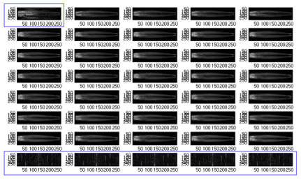
Fig. 1 All frames in the original series. Frames circled in blue will be discarded as noise frames.
As mentioned earlier, what we are really interested in is the resulted image by subtracting a mask image from a phase image which shows the vasculature. Figure 2 shows an example of such subtraction. When two unmatched images are subtracted, the vasculature would not be revealed as shown in Fig.2 (d).

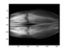
(a) Mask (b) Phase
(c) Subtracted Image (d) inappropriate mask & phase match
Fig.2 An example of phase and mask images and the corresponding subtracted image. Also an example of subtracted image due to inappropriate match of frames.
Proposed Experiment
Supervised learning is our first consideration; however, as mentioned earlier, we do not have any labels for each patient, each frame, or each pixel. There is one possibility of learning the arrival of contrast, however with only fifteen patients and thirty frames per patient, the amount of data is too scarce for supervised learning. In addition, the fact that the labels are human or computer estimations makes this proposal less desirable. Moreover, this problem has been well studied and fully automated algorithm that accurately estimates the contrast arrival has been devised, which leaves little value in studying this particular problem further.
While we do not have sufficient data at patient level, or frame level, we propose an experiment to attempt unsupervised learning at pixel level of subtracted images by building profile on each pixel in a modified notion of time series. This profile is analogous to the voxel profile in fMRI clustering done in Goutte et al. (1999 ) and Mitchell et al. (2004). We hypothesize that by doing clustering on these pixels, the pixels where the arteries reside can be identified, which can be a valuable enhancement information for the current developed algorithm for automatic selection of mask and phase images. We also hypothesized that the clusters might reveal a trace of the contrast.
Method
For n frames, we use the first five frames as masks, and all immediate subsequent frames (including the masks) in the series as phase images. The subtraction results in k = 5(n – 3) subtracted images. The profile for each pixel (x, y) is the vector of intensities of these k images therefore we have a x by y by k matrix. Each of these vectors is analogous to a cell in a MicroArray chip. The notion of time series is however slightly different from the ones in fMRI because by subtracting different masks, we ‘go back’ in time recurrently. Due to the computing resource we have and time constrain, we were forced to filter the data points from all 77352 pixels to about 7000. It is very expensive to calculate the pair-wise correlation; it takes roughly 20 hours to compute for 7000 points which results in 24496500 pairs of data points. The filtering was accomplished by calculating the variance of each vector and the vectors with the highest 7000 variances were included to be clustered. This filtering process does not affect the result as we assume the background pixels, the pixels we are not interested, have relatively constant variance. Figure 4 and 5 shows the original and sorted variance of the profile over each pixel. We verify and confirm our assumption by plotting the pixels chosen. It can be seen from Figure 6 that we do not lose vasculature and in fact the structure of the vasculature can already be vaguely sketched out.
Finally, we base our definition of pair-wise distance between every chosen pixel by calculating the Centered Pearson Correlation S:
![]()
![]()
where X and Y are the two vectors, N is the size of the vector, and the offset is the mean of the vector. S is bounded by -1 and 1 where negative values correspond to negative correlation and positive values correspond to positive correlation. The stronger the correlation is the closer S is to 1 or -1. What we are really interested in and also what the package requires is the distance between two pixels. Distance should be positive and larger when the two pixels are less correlated and vice versa. Therefore we convert all correlations S to D where D = 1 – abs(S) which makes D fulfill our desire distance property.
We have chosen to use agglomerative algorithm to build hierarchical clustering. Unlike k-means algorithm where the number of cluster is preset, agglomerative algorithm produces clusters at all n levels where n is the number of data points, 7000 in our case. This property allows us to view results in different clustering levels, different number of clusters, which might reveal different meaningful underlying fundamental structure of the data. By default, for every level we merge two clusters that have the smallest average pair-wise distance. We also experiment with nearest neighboring distance, that is to merger the pair of clusters that has the closest two single data points. Finally we pick the ‘interesting’ clusters by choosing the cluster that is just about to have a significant jump on its weighted sum of internal distance which is a measurement that shows how compact the overall clustering is. We choose such clusters because a jump in the weighted sum of internal distance signifies two very distinct clusters are to be joined. Figure 7 shows an example of how we choose the interesting clusters. The following figure pictorially shows the flow of how we obtain the profiles used in clustering the pixels.
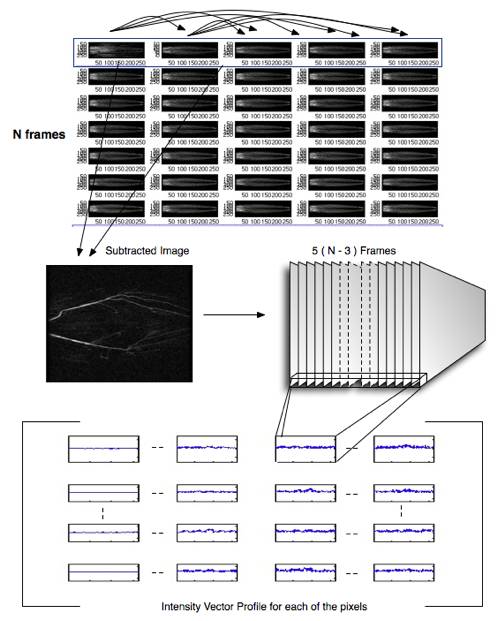
Fig. 3 Pictorially showing the data gathering flow.
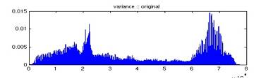
Fig. 4 Intensity variance of each profile over a pixel.
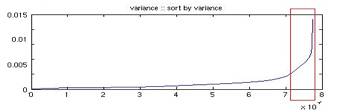
Fig. 5 Sorted intensity variance of each profile over a pixel.
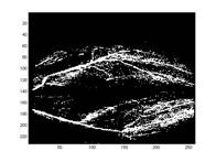
Fig. 6 7000 highest variance pixels located on the map. These points correspond to the red circled area in Fig. 5.
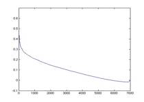
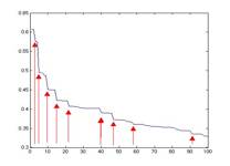
Fig. 7 Number of Clusters V.S. Weighted Sum of Internal Distance, red arrows shows cluster of interest.
Results
5 Clusters 10 Clusters
28 Clusters 47 Clusters

50 Clusters 58 Clusters
65 Clusters 68 Clusters
82 Clusters 98 Clusters
179 Clusters 225 Clusters
251 Clusters 289 Clusters
1277 Clusters
1787 Clusters
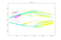
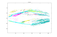
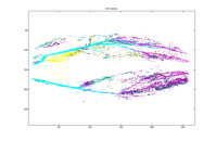
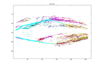
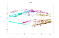
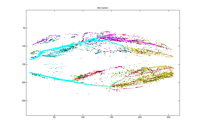
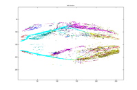
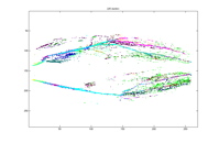
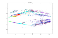
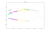
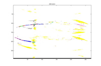
Each of the graphs above shows the
clusters made by the agglomerative algorithm. Every graph shows 28 largest
clusters and every color is mapped to one cluster. It can be seen that with
five clusters, although one major branch for the left leg is missed, other major
vessels are quite clearly sketched out with their almost entirety from the top
to the end. The major spine of the vessel is caught into one cluster very
early on, when there are still more than a thousand clusters. Another
interesting phenomenon to point is how the clusters segment the major vessels into
three major pieces in early stages. We suspect this can be the trace of the
contrast. As the number of the clusters decrease, the vessel continues to be
segmented into at least two major pieces as seen with 50 or 47 clusters.
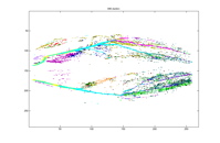
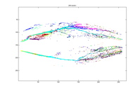
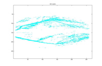
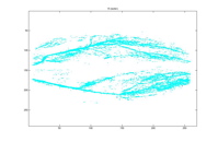
2 Clusters 3 Clusters
153 Clusters 2669 Clusters
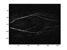
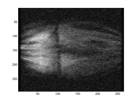
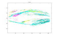
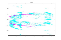
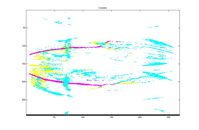
Here we show the results of a different patient. For this particular patient although the major vessels are sketched out, unfortunately the lower extreme is blended into other clusters. However this patient shows some other unexpected effect of clustering, that is to distinguish motion artifacts from the vessels. These are artifacts that result from the motion of the patient during the course of MR data gathering. Because the data is gathered in k-space, motion results in multiple ‘phantom’ copies in the image. Figure 8 shows an example of motion artifacts in a real subtracted image. Traditionally, the pixels of the motion artifacts are very difficult to be distinguished from other vessel pixels, because the intensities are very similar to the ones of vasculature; here we can clearly see that the artifacts are caught into one cluster very early on. Unfortunately, the lower extremes of the actual vessel is eventually confused with the artifacts.
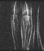 Fig 8. An example
of motion artifacts.
Fig 8. An example
of motion artifacts.
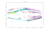
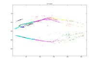
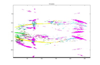
1801 Clusters 15 Clusters
As mentioned earlier, besides using minimum average distance, we also experience nearest neighboring distance. It can be seen from the above two plots the result is quite poor. Even very early on, the pixels are completely incorrectly clustered. Since agglomerative clustering makes new cluster by grouping existing clusters, this misleading cluster persisted in the remaining levels of clusters.
Application
With 30 to 40 MR images per patient, the number of mask and phase image pairs is too large for manual selection process to exhaust all possible matches. Computer algorithm has been developed to automate this process which may examine every single mask and phase image match in a reasonable amount of time and provide clinician with the pair that results the best subtracted image. The most important step in the process is to score each subtracted image and the scoring function is usually the intensity contrast between the vasculature and the background i.e. the sum of intensity of the vasculature should be as high as possible where the intensity of the background should be as low as possible. The reliability of this scoring function highly depends on the correct identification of the vasculature pixels. Current algorithms predict the pixels by static properties of each subtracted images with certain assumptions of the structure of the vasculature.
As it can be seen from the result, without any prior knowledge or assumption of the vasculature, clustering is able to sketch out a very clear boundary of the vasculature by collecting the intensity profile over a series of images. Although the pixels identified as vessels might not be correct for any specific subtracted image, it can still be used as a helpful hint to whether a pixel should be labeled as foreground, in turn enhance the quality of automatic selection algorithm.
Conclusion & Future Direction
This project has shown one possible application of unsupervised learning in the domain of CEMRA. With no prior information or assumption, clustering is able to reveal some structures of the CEMRA images. The result has shown that by using the intensity profile over a series of subtracted images, clustering may show the major vessels in angiography images. Moreover, by using agglomerative clustering, we were able to examine the different clusters with different cluster level. With such information, we see how the major vessels are segmented (perhaps logically) and we hypothesize this could be an indication of the trace of the contrast. In addition, we unexpectedly see how clustering can distinguish motion artifacts from actual vessels. This effect might have the potential value in enhancing image quality when undesirable artifacts persist in the image sequence.
While this experiment is a rough and more of a feasibility experiment, a number of more refined subsequent experiments may be attempted in the future. In this particular experiment we arbitrarily chose five mask images to subtract. One may experiment with different number of masks, from one to, perhaps, the frame where contrast is estimated to arrive and see if this affects the result. Secondly, more data is better. Due to time and computing resource constrain, we were only able to collect pair wise correlation over 7000 points, which is a significantly small portion of the image. It would be interesting to see how with additional data points, more or better information may be revealed. Moreover, some other distance metrics may be devised; if the metric can be more sensitive, perhaps the smaller the vessels may also be accurately identified. Last but not least, instead of clustering pixels in the images, one may attempt to cluster the subtracted images. This is an entire different problem, however it may be another potential application of unsupervised learning in the CEMRA domain.
Reference
1. Goutte, C. et al. On Clustering fMRI Time Series. Neuro Image 9:298-310(1999)
2. Kim, J. et al. Automatic Selection of Mask and Arterial Phase Images for Temporally Resolved MR Digital Subtraction Angiography. Magnetic Resonance in Medicine 48:1004-1010(2002)
3. Kuo, Yuan-Fen. A New Approach in Foreground Identification for Quality Evaluation of Temporally Resolved MR Digital Subtraction Angiography
4. Mitchell, T. et al. Learning to Decode Cognitive States from Brain Images. Machine Learning 57:145-175(2004)
5. https://genome.unc.edu/MicroArray/help/analysis.shtml
Appreciation
Many special thanks to Prof. Rich Caruana for spending time to support, advise and provide the clustering package.