]>

Simpson's Method for numerical integration

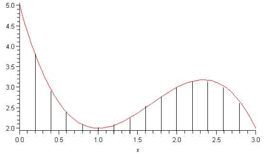
Numerical integration uses the concept that a definite integral of a function between two limits is simply the “area under the curve”. The only complication is estimating the integrand function. Of course if you knew the function that was the integral of the integrand function you would not have to do a numerical integral; you could do it analytically. Simpson’s Method breaks the interval between the limits into a number of subintervals that you specify and then approximates the function in each subinterval as a quadratic polynomial that passes through the two end points and the mid-point of the subinterval. You know how to integrate a quadratic polynomial, so then you just add up the integrals of all the quadratic polynomials that approximate the integrands in each subinterval to get the total integral. For smooth well behaved integrands, if you choose enough narrow subintervals, then this is a good approximation to the area under the curve. This is shown graphically in the figure below for the function

f ( x ) = ( x 1 ) 3 + 2 ( x 1 ) 2 + 2 MathType@MTEF@5@5@+=feaafiart1ev1aaatCvAUfeBSjuyZL2yd9gzLbvyNv2CaerbuLwBLnhiov2DGi1BTfMBaeXatLxBI9gBaerbd9wDYLwzYbItLDharqqtubsr4rNCHbGeaGqiVu0Je9sqqrpepC0xbbL8F4rqqrFfpeea0xe9Lq=Jc9vqaqpepm0xbba9pwe9Q8fs0=yqaqpepae9pg0FirpepeKkFr0xfr=xfr=xb9adbaqaaeGaciGaaiaabeqaamaabaabaaGcbaGaamOzamaabmaabaGaamiEaaGaayjkaiaawMcaaiabg2da9iabgkHiTmaabmaabaGaamiEaiabgkHiTiaaigdaaiaawIcacaGLPaaadaahaaWcbeqcbaAaaiaaiodaaaGccqGHRaWkcaaIYaWaaeWaaeaacaWG4bGaeyOeI0IaaGymaaGaayjkaiaawMcaamaaCaaaleqajeaObaGaaGOmaaaakiabgUcaRiaaikdaaaa@4A24@ between the limits x = 0 MathType@MTEF@5@5@+=feaafiart1ev1aaatCvAUfeBSjuyZL2yd9gzLbvyNv2CaerbuLwBLnhiov2DGi1BTfMBaeXatLxBI9gBaerbd9wDYLwzYbItLDharqqtubsr4rNCHbGeaGqiVu0Je9sqqrpepC0xbbL8F4rqqrFfpeea0xe9Lq=Jc9vqaqpepm0xbba9pwe9Q8fs0=yqaqpepae9pg0FirpepeKkFr0xfr=xfr=xb9adbaqaaeGaciGaaiaabeqaamaabaabaaGcbaGaamiEaiabg2da9iaaicdaaaa@38AA@ and x = 3 MathType@MTEF@5@5@+=feaafiart1ev1aaatCvAUfeBSjuyZL2yd9gzLbvyNv2CaerbuLwBLnhiov2DGi1BTfMBaeXatLxBI9gBaerbd9wDYLwzYbItLDharqqtubsr4rNCHbGeaGqiVu0Je9sqqrpepC0xbbL8F4rqqrFfpeea0xe9Lq=Jc9vqaqpepm0xbba9pwe9Q8fs0=yqaqpepae9pg0FirpepeKkFr0xfr=xfr=xb9adbaqaaeGaciGaaiaabeqaamaabaabaaGcbaGaamiEaiabg2da9iaaiodaaaa@38AD@ .

Simpson Graph

If you fit the three points in each subinterval to a quadratic polynomial then integrate each of these and then add them together you get the formula

a b f ( x ) d x h 3 [ f ( x 0 ) + 4 f ( x 1 ) + 2 f ( x 2 ) + 4 f ( x 3 ) + 2 f ( x N 2 ) + 4 f ( x N 1 ) + f ( x N ) ] MathType@MTEF@5@5@+=feaafiart1ev1aaatCvAUfeBSjuyZL2yd9gzLbvyNv2CaerbuLwBLnhiov2DGi1BTfMBaeXatLxBI9gBaerbd9wDYLwzYbItLDharqqtubsr4rNCHbGeaGqiVu0Je9sqqrpepC0xbbL8F4rqqrFfpeea0xe9Lq=Jc9vqaqpepm0xbba9pwe9Q8fs0=yqaqpepae9pg0FirpepeKkFr0xfr=xfr=xb9adbaqaaeGaciGaaiaabeqaamaabaabaaGcbaWaa8qCaeaacaWGMbWaaeWaaeaacaWG4baacaGLOaGaayzkaaGaamizaiaadIhaaSqaaiaadggaaeaacaWGIbaaniabgUIiYdGccqGHijYUdaWcaaqaaiaadIgaaeaacaaIZaaaamaadmaabaGaamOzamaabmaabaGaamiEamaaBaaaleaacaaIWaaabeaaaOGaayjkaiaawMcaaiabgUcaRiaaisdacaWGMbWaaeWaaeaacaWG4bWaaSbaaSqaaiaaigdaaeqaaaGccaGLOaGaayzkaaGaey4kaSIaaGOmaiaadAgadaqadaqaaiaadIhadaWgaaWcbaGaaGOmaaqabaaakiaawIcacaGLPaaacqGHRaWkcaaI0aGaamOzamaabmaabaGaamiEamaaBaaaleaacaaIZaaabeaaaOGaayjkaiaawMcaaiabgUcaRiabl+UimjaaikdacaWGMbWaaeWaaeaacaWG4bWaaSbaaSqaaiaad6eacqGHsislcaaIYaaabeaaaOGaayjkaiaawMcaaiabgUcaRiaaisdacaWGMbWaaeWaaeaacaWG4bWaaSbaaSqaaiaad6eacqGHsislcaaIXaaabeaaaOGaayjkaiaawMcaaiabgUcaRiaadAgadaqadaqaaiaadIhadaWgaaWcbaGaamOtaaqabaaakiaawIcacaGLPaaaaiaawUfacaGLDbaaaaa@7216@

where you divide the interval [ a , b ] MathType@MTEF@5@5@+=feaafiart1ev1aaatCvAUfeBSjuyZL2yd9gzLbvyNv2CaerbuLwBLnhiov2DGi1BTfMBaeXatLxBI9gBaerbd9wDYLwzYbItLDharqqtubsr4rNCHbGeaGqiVu0Je9sqqrpepC0xbbL8F4rqqrFfpeea0xe9Lq=Jc9vqaqpepm0xbba9pwe9Q8fs0=yqaqpepae9pg0FirpepeKkFr0xfr=xfr=xb9adbaqaaeGaciGaaiaabeqaamaabaabaaGcbaGaai4waiaadggacaGGSaGaamOyaiaac2faaaa@3A2A@ into N MathType@MTEF@5@5@+=feaafiart1ev1aaatCvAUfeBSjuyZL2yd9gzLbvyNv2CaerbuLwBLnhiov2DGi1BTfMBaeXatLxBI9gBaerbd9wDYLwzYbItLDharqqtubsr4rNCHbGeaGqiVu0Je9sqqrpepC0xbbL8F4rqqrFfpeea0xe9Lq=Jc9vqaqpepm0xbba9pwe9Q8fs0=yqaqpepae9pg0FirpepeKkFr0xfr=xfr=xb9adbaqaaeGaciGaaiaabeqaamaabaabaaGcbaGaamOtaaaa@36C0@ subintervals and N MathType@MTEF@5@5@+=feaafiart1ev1aaatCvAUfeBSjuyZL2yd9gzLbvyNv2CaerbuLwBLnhiov2DGi1BTfMBaeXatLxBI9gBaerbd9wDYLwzYbItLDharqqtubsr4rNCHbGeaGqiVu0Je9sqqrpepC0xbbL8F4rqqrFfpeea0xe9Lq=Jc9vqaqpepm0xbba9pwe9Q8fs0=yqaqpepae9pg0FirpepeKkFr0xfr=xfr=xb9adbaqaaeGaciGaaiaabeqaamaabaabaaGcbaGaamOtaaaa@36C0@ is even. You can see the pattern of coefficients 1, 4, 2, 4, 2, 4, 2, …, 2, 4, 1 and x 0 = a MathType@MTEF@5@5@+=feaafiart1ev1aaatCvAUfeBSjuyZL2yd9gzLbvyNv2CaerbuLwBLnhiov2DGi1BTfMBaeXatLxBI9gBaerbd9wDYLwzYbItLDharqqtubsr4rNCHbGeaGqiVu0Je9sqqrpepC0xbbL8F4rqqrFfpeea0xe9Lq=Jc9vqaqpepm0xbba9pwe9Q8fs0=yqaqpepae9pg0FirpepeKkFr0xfr=xfr=xb9adbaqaaeGaciGaaiaabeqaamaabaabaaGcbaGaamiEamaaBaaaleaacaaIWaaabeaakiabg2da9iaadggaaaa@39C6@ and x N = b MathType@MTEF@5@5@+=feaafiart1ev1aaatCvAUfeBSjuyZL2yd9gzLbvyNv2CaerbuLwBLnhiov2DGi1BTfMBaeXatLxBI9gBaerbd9wDYLwzYbItLDharqqtubsr4rNCHbGeaGqiVu0Je9sqqrpepC0xbbL8F4rqqrFfpeea0xe9Lq=Jc9vqaqpepm0xbba9pwe9Q8fs0=yqaqpepae9pg0FirpepeKkFr0xfr=xfr=xb9adbaqaaeGaciGaaiaabeqaamaabaabaaGcbaGaamiEamaaBaaaleaacaWGobaabeaakiabg2da9iaadkgaaaa@39E0@ . The subinterval width is h = b a N MathType@MTEF@5@5@+=feaafiart1ev1aaatCvAUfeBSjuyZL2yd9gzLbvyNv2CaerbuLwBLnhiov2DGi1BTfMBaeXatLxBI9gBaerbd9wDYLwzYbItLDharqqtubsr4rNCHbGeaGqiVu0Je9sqqrpepC0xbbL8F4rqqrFfpeea0xe9Lq=Jc9vqaqpepm0xbba9pwe9Q8fs0=yqaqpepae9pg0FirpepeKkFr0xfr=xfr=xb9adbaqaaeGaciGaaiaabeqaamaabaabaaGcbaGaamiAaiabg2da9maalaaabaGaamOyaiabgkHiTiaadggaaeaacaWGobaaaaaa@3B7D@ . The beauty of this formula is that the approximation error associated with using finite subinterval width h MathType@MTEF@5@5@+=feaafiart1ev1aaatCvAUfeBSjuyZL2yd9gzLbvyNv2CaerbuLwBLnhiov2DGi1BTfMBaeXatLxBI9gBaerbd9wDYLwzYbItLDharqqtubsr4rNCHbGeaGqiVu0Je9sqqrpepC0xbbL8F4rqqrFfpeea0xe9Lq=Jc9vqaqpepm0xbba9pwe9Q8fs0=yqaqpepae9pg0FirpepeKkFr0xfr=xfr=xb9adbaqaaeGaciGaaiaabeqaamaabaabaaGcbaGaamiAaaaa@36DA@ varies as h 4 MathType@MTEF@5@5@+=feaafiart1ev1aaatCvAUfeBSjuyZL2yd9gzLbvyNv2CaerbuLwBLnhiov2DGi1BTfMBaeXatLxBI9gBaerbd9wDYLwzYbItLDharqqtubsr4rNCHbGeaGqiVu0Je9sqqrpepC0xbbL8F4rqqrFfpeea0xe9Lq=Jc9vqaqpepm0xbba9pwe9Q8fs0=yqaqpepae9pg0FirpepeKkFr0xfr=xfr=xb9adbaqaaeGaciGaaiaabeqaamaabaabaaGcbaGaamiAamaaCaaaleqabaGaaGinaaaaaaa@37C5@ Thus if you halve the value of h MathType@MTEF@5@5@+=feaafiart1ev1aaatCvAUfeBSjuyZL2yd9gzLbvyNv2CaerbuLwBLnhiov2DGi1BTfMBaeXatLxBI9gBaerbd9wDYLwzYbItLDharqqtubsr4rNCHbGeaGqiVu0Je9sqqrpepC0xbbL8F4rqqrFfpeea0xe9Lq=Jc9vqaqpepm0xbba9pwe9Q8fs0=yqaqpepae9pg0FirpepeKkFr0xfr=xfr=xb9adbaqaaeGaciGaaiaabeqaamaabaabaaGcbaGaamiAamaaCaaaleqabaaaaaaa@3707@ (i.e. choose twice as many subintervals) then the error is reduced by 2 4 MathType@MTEF@5@5@+=feaafiart1ev1aaatCvAUfeBSjuyZL2yd9gzLbvyNv2CaerbuLwBLnhiov2DGi1BTfMBaeXatLxBI9gBaerbd9wDYLwzYbItLDharqqtubsr4rNCHbGeaGqiVu0Je9sqqrpepC0xbbL8F4rqqrFfpeea0xe9Lq=Jc9vqaqpepm0xbba9pwe9Q8fs0=yqaqpepae9pg0FirpepeKkFr0xfr=xfr=xb9adbaqaaeGaciGaaiaabeqaamaabaabaaGcbaGaaGOmamaaCaaaleqabaGaaGinaaaaaaa@3794@ or 16 over the error in the original estimate. Simpson’s Method is called a fourth order accurate numerical algorithm because of this property.

Simpson’s Method is an example of the type of method used for numerically estimating definite integrals by the int(f,x=a..b,numeric) command in Maple and quad function in Matlab. While these do not use Simpson’s Method specifically, they use more sophisticated methods that are similar in principle.