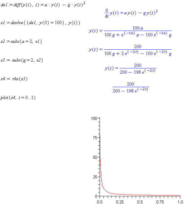
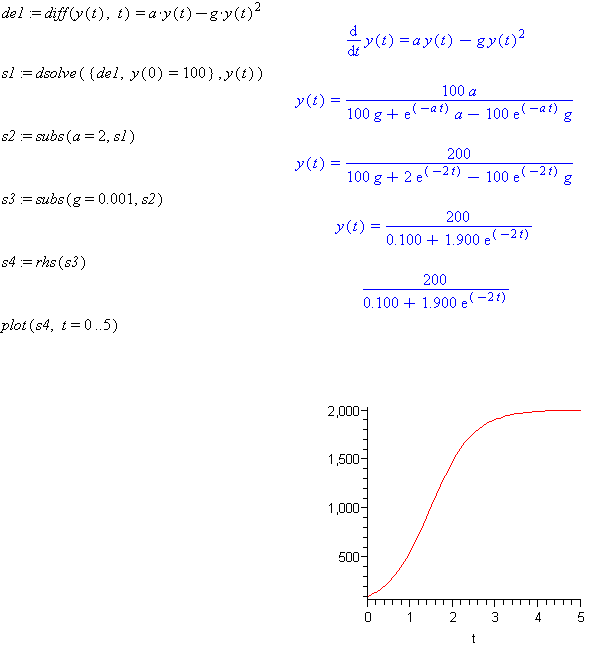
Examples:
         de1:=diff(y(t), t) = a*y(t)-g*y(t)^2
s1:=dsolve({de1, y(0)=100},y(t))
s2:=subs(a=2, s1)
s3:=subs(g=2, s2)
s4:=rhs(s3)
plot(s4, t=0..1)
          de1:=diff(y(t), t) = a*y(t)-g*y(t)^2
s1:=dsolve({de1, y(0)=100},y(t))
s2:=subs(a=2, s1)
s3:=subs(g=0.001, s2)
s4:=rhs(s3)
plot(s4, t=0..5)
Note: All that changed in the ODE for this example is g but the graph is drastically different.
Now we will do the same problem but use right-click instead.
Enter:y'=alpha*y-g*y^2
Right-click and select solve DE interactively
Click edit under the Conditions box and enter 0 and 100 so the top reads y at 0=100 and then click edit under parameters and enter 2 for alpha and g
Now click Solve Symbolically
Click Solve on the top right of the window that opens and then on the bottom left select 'on Quit, Return Solution'
Now click Quit in the bottom right
Right click the returned solution and hit Right-Hand Side
Right click and select plot->2D
Right click and change the range to 0 to 1 for the x and make appropriate changes to the y axis.
Now we will do the same problem but with a different value of g
Enter:y'=alpha*y-g*y^2
Right-click and select solve DE interactively
Click edit under the Conditions box and enter 0 and 100 so the top reads y at 0=100 and then click edit under parameters and enter 2 for alpha and 0.0001 for g
Now click Solve Symbolically
Click Solve on the top right of the window that opens and then on the bottom left select 'on Quit, Return Solution'
Now click Quit in the bottom right
Right click the returned solution and hit Right-Hand Side
Right click and select plot->2D
Right click and change the range to 0 to 10 for the x and make appropriate changes to the y axis.

