Examples:

1. Find the numeric solution of this ODE when f(0)=3, then find the value of the solution at x=15, and finally plot the solution procedure. $$\frac{df(x)}{dx}=-\frac{f{(x)}^2}{5}$$

         > soln1 := dsolve({diff(f(x),x) = -(1/5)*f(x)^2, f(0)=3}, f(x), numeric)
         > soln1(5)
         > with(plots):
         > odeplot(soln1,[x,f(x)],x=0..8)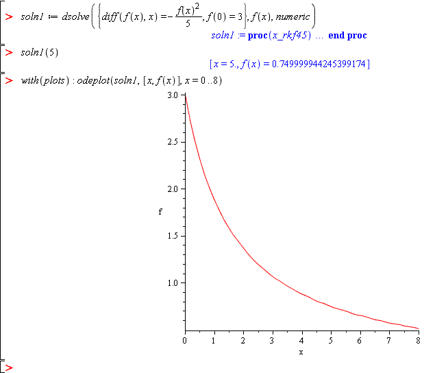
   

   

   Contrast the Maple command soln1(15) to find the value of a numeric solution when x=15 with using the subs(x=15,soln) command to find such a value of a symbolic solution.

2. We will now solve the problem of rabbit and fox populations (using Maple commands) and look at graphs over a long time period. First, try to solve the problem symbolically for initial conditions r(0)=r₀ and f(0)=f₀. Try these commands in a Maple worksheet:

   rODE := diff(r(t),t) = alpha*r(t) - beta*r(t)*f(t)
   fODE := diff(f(t),t) = -gamma*f(t) + delta*r(t)*f(t)
   odeSoln := dsolve({rODE,fODE,r(0)=r0,f(0)=f0},{r(t),f(t)})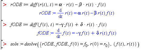
   

   

3. Since Maple was unable to symbolically solve this problem, we must solve it numerically. Use initial conditions r(0)=400 and f(0)=16 and parameters alpha=1.6, beta=0.11, delta=0.01, and gamma=3.7.

   Add these commands to those above:

   odeSystem := subs(alpha=1.6, beta=0.11,gamma=3.7, delta=0.01, {rODE,fODE,r(0)=400,f(0)=16} )
   odeSoln := dsolve(odeSystem,{r(t),f(t)},numeric)
   

   

   The numeric solution is a set of points. However, Maple returns it as a procedure that you can now use to compute values at any desired point in time.

4. Find the number of rabits and foxes at t=10. To do this, simply pass the value 10 as an argument to the newly created function. Type odeSoln(10) and see the result.

   

   Notice, that the value of t, and the values for r(t), and f(t) are all returned by this single solution procedure.

5. Plot the solution function, from t=0..10, using the odeplot command. Add the option, numPoints=20000 to your odeplot command. Note: If you haven't executed with(plots) since the last restart, you will need to execute that command also.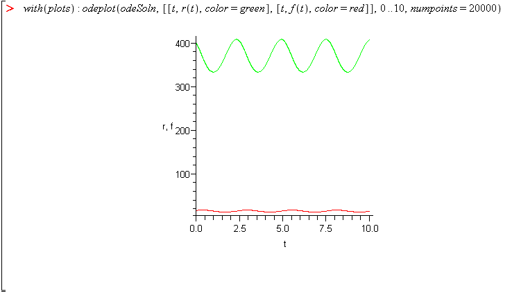

   

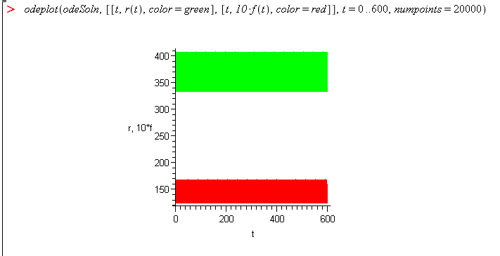
   Note: The syntax for the odeplot command that plots the numeric solution is different from the earlier plot commands covered in the course.

6. Plot the solution over the range from 0 to 600 with 20000 points to get a more continuous curve.

   Note: Notice that the two functions look like two wide bands because the solution is varying very rapidly. We look at the graph at shorter increments to see the behavior.

   

7. Note: To more clearly see the behavior, multiply the fox function by 10 and plot only 10% of the plot, change the range to 540-600.

   

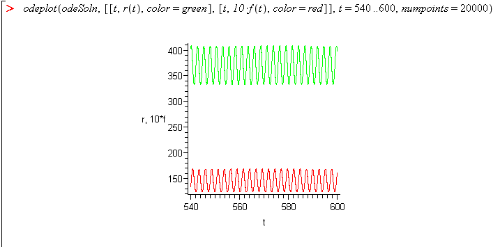
   The fox value is multiplied by 10 to make it easier to see along with the much larger rabbit population.

8. To clearly see the behavior of 1% of the plot, plot only the range to 594-600.

   

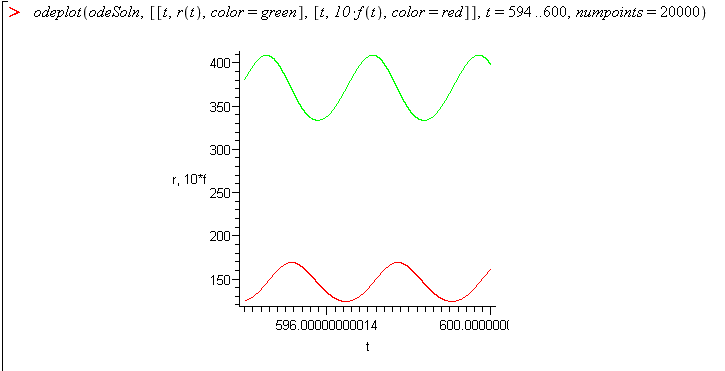
   Here we notice that as the fox population increases, the rabbit population peaks and starts to decrease and the fox population peaks and decreases as the rabbit population decreases. This is caused by the relationship that the more foxes, the more rabbits eaten, and the more rabbits, the more food to produce more foxes. We can further alter this model by adding other factors like disease or habitat destruction.

9. Now we will solve the same Rabbit-Fox problem but by using the ODE analyzer.
   Note: The use of the ODE Analyzer will not be covered on the exams.

   To access ODE Analyzer, do one of the following:

   • Type dsolve[interactive](); on a command line of your worksheet or document or
   • Use the menu option: Tools -> Assistants -> ODE analyzer

   After the analyzer window is open, enter the ODEs, initial conditions with values, the value of any parameters (variables), and click Solve Numerically. You will also have to specify all parameters for the numerical solution to work. After you’ve entered all the required information into the ODE analyzer, click Solve Numerically in the bottom left of the analyzer screen.

   

   Note: First assign the two equations to variables and then open ODE analyzer.

   

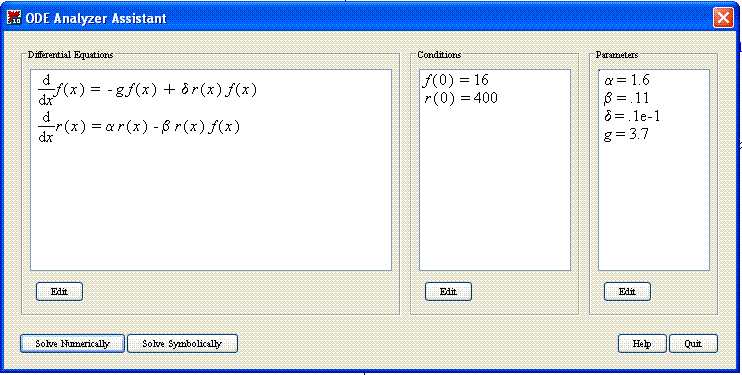
   Note: Input the expressions, parameters and conditions and then click Solve Numerically in the bottom left of the window

   

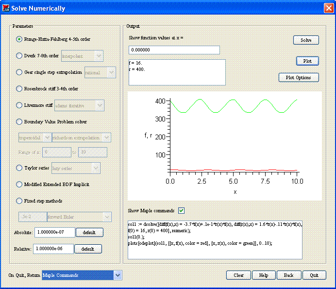
   Notice the list on the left of the ODE Analyzer window, there are different numerical methods you can select to solve the problem. The default method is already selected, and is Runge-Kutta-Fehlberg 4-5th order. This is the usually the best option for solving these types of problems numerically.

   The Solve Numerically window can perform many different operations. If you put a value in the box under "Show function values at x=" and click Solve, the values of your functions will be displayed. You can plot in this window by hitting plot and can change the options of the plot by clicking plot options. These tools allow for finding selected points and provide a visual representation of what the full solution looks like.

   

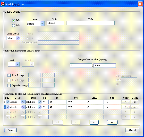
   Note: Change the range of x to 0 to 1500 and copy the function and change the 2nd function to r. Then click done. In the ODE analyzer hit plot then change return to the maple commands and hit done.

   

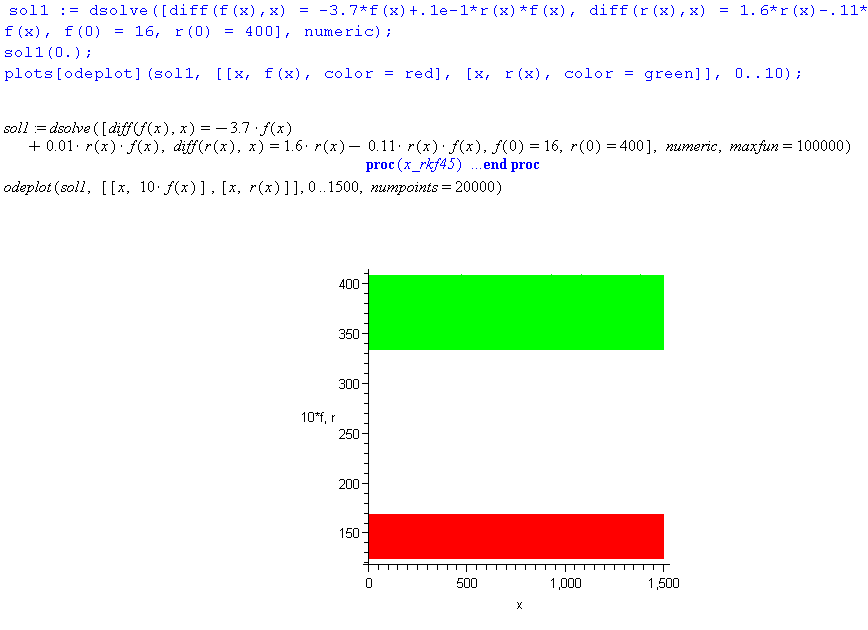
   Note: Rewrite the first line returned back into Maple and add maxfun=10000 to the end of the command and hit enter. Then type odeplot(sol1, [[x, 10*f(x)], [x, r(x)]], 0 .. 1500, numpoints = 20000) where 0..1500 sets the range and numpoints=20000 means there will be 20000 points plotted, much less doesn't show the real behavior of the functions.
   We'll look at the graph at shorter increments to see the behavior (as we did in example 1).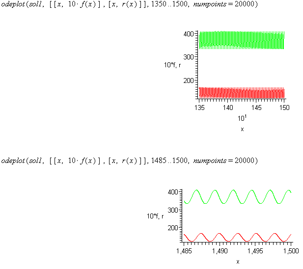

   

   You can return the values you compute or the plot you make to the underlying document or worksheet. Then, you will be able to edit it in the document. Also, you can return the Numeric Procedure to the document. This is the procedure that would have been returned had you typed the dsolve command in the document. The procedure is assigned a name so that values of the solution can be found as if the name was a function.

   However, there are some limits on using this window. It is therefore necessary to understand and be able to use the dsolve directly, as shown earlier.