]> Exercises

Exercises

Solve each ODE both analytically and numerically. Also, plot the analytical and numerical solutions.

  1. d y d t = 2 t y      y(0)=10 MathType@MTEF@5@5@+=feaafiart1ev1aaatCvAUfeBSjuyZL2yd9gzLbvyNv2CaerbuLwBLnhiov2DGi1BTfMBaeXatLxBI9gBaerbd9wDYLwzYbItLDharqqtubsr4rNCHbGeaGqiVu0Je9sqqrpepC0xbbL8F4rqqrFfpeea0xe9Lq=Jc9vqaqpepm0xbba9pwe9Q8fs0=yqaqpepae9pg0FirpepeKkFr0xfr=xfr=xb9adbeqabeWacmGabiqabeqabmaabaabaaGcbaWaaSaaaeaacaWGKbGaamyEaaqaaiaadsgacaWG0baaaiabg2da9iaaikdacaWG0bGaamyEaiaabccacaqGGaGaaeiiaiaabccacaqGGaGaaeyEaiaabIcacaqGWaGaaeykaiaab2dacaqGXaGaaeimaaaa@45E2@

    Hint: The solution changes quickly, choose your range of t for the plot carefully.

    To get the analytical solution
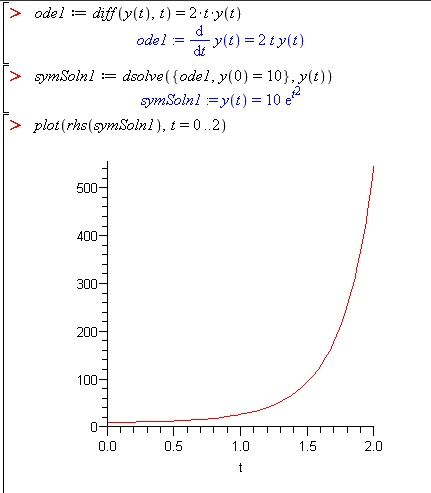
    exponentially increasing function as t get larger

    Note: I had to plot from 0 to 2 because if you set the range beyond a certain point y is increasing so fast that Maple can not plot the values. Also, there isn't additional behavior detail when plotting over a larger range.

    To get the numerical solution
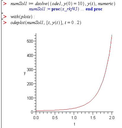
    exponentially increasing function as t get larger

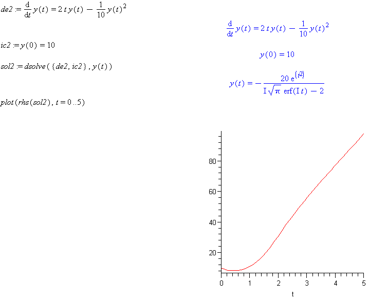
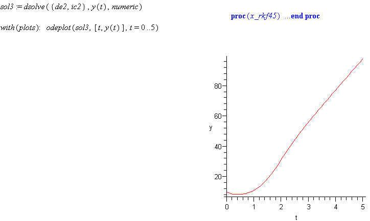
  2. d y d t = 2 t y y ( t ) 2 10        y ( 0 ) = 10 MathType@MTEF@5@5@+=feaafiart1ev1aaatCvAUfeBSjuyZL2yd9gzLbvyNv2CaerbuLwBLnhiov2DGi1BTfMBaeXatLxBI9gBaerbd9wDYLwzYbItLDharqqtubsr4rNCHbGeaGqiVu0Je9sqqrpepC0xbbL8F4rqqrFfpeea0xe9Lq=Jc9vqaqpepm0xbba9pwe9Q8fs0=yqaqpepae9pg0FirpepeKkFr0xfr=xfr=xb9adbeqabeWacmGabiqabeqabmaabaabaaGcbaWaaSaaaeaacaWGKbGaamyEaaqaaiaadsgacaWG0baaaiabg2da9iaaikdacaWG0bGaamyEaiabgkHiTmaalaaabaGaamyEaiaacIcacaWG0bGaaiykamaaCaaaleqabaGaaGOmaaaaaOqaaiaaigdacaaIWaaaaiaabccacaqGGaGaaeiiaiaabccacaqGGaGaaeiiaiaadMhacaGGOaGaaGimaiaacMcacqGH9aqpcaaIXaGaaGimaaaa@4D99@

    To get the analytical solution

    Maple Screenshot

    To get the numerical solution

    Maple Screenshot