Numerical solutions of ordinary differential equations

What does it mean to solve a differential equation numerically? Recall that the solution of an ODE is a function, y(t). A function y(t) is fundamentally a set of points having the form (t,y(t)). When we talk about a numerical solution to an ODE, we mean a large list of (t,y) points where the y in each point is approximately equal to y(t).

To find these solutions, we start by looking at our general form of the ODE:

$\frac{d y (t)}{d t} = F (t, y (t))$ , initial condition $y (t_{0}) = y_{0}$ , and $F (t, y (t))$ is some combination of terms involving the independent variable t and the unknown function y(t).

Numerical solutions of ODE's start with what we know, the initial condition $y (t_{0}) = y_{0}$ , and use this and the ODE itself to estimate the function at a nearby point. The ODE allows us to compute the derivative of the unknown function at the point $(t_{0}, y (t_{0}))$ because

$y' (t_{0}) = F (t_{0}, y_{0})$

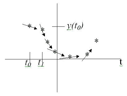
we use this derivative as the slope to give a direction in which to estimate the next point of the numerical solution $(t_{1}, y (t_{1}))$ . This is done over and over until an approximation to the function is known over the total domain of interest. The result of this process is pairs of points $t_{k}$ and $y (t_{k}) = y_{k}$ , k=0,1,2,.... The following figure gives a graphical explanation of the idea behind the numerical solution of ODE's.

Maple Screenshot

We know $t_{0}$ and $y (t_{0})$ and we know the slope of y(t), y' given as y'=F(t,y).
We don't know y(t) for any values of t other than $t_{0}$ .

We will describe how to obtain approximate solutions to ODE's using a class of methods called Runge-Kutta methods. (There are other numerical techniques for solving ODE's that we will not discuss.) We consider the equation from an initial time $t_{0}$ up to some later time $t_{e n d}$ . We choose a time step $Δ t = t_{1} - t_{0}$ , often denoted in mathematics texts as h. The solution is computed at the discrete times $t_{k} = t_{0} + k h$ for k=0,1,2.... The approximate solution at time $t_{k}$ will be denoted by $y_{k}$ . Note that a numerical solution to a differential equation is a table of numbers, each of which gives an approximation to the true solution at each time $t_{k}$ . This is to be distinguished from the exact analytical solution, which is a continuous function.

The first method we will discuss is called Euler's method, named after a famous mathematician named Euler (pronounced "Oiler"). Euler's method is obtained by approximating the derivative at time $t_{k}$ with a simple difference. The approximating equation is

$\frac{d y}{d t} \approx \frac{y_{k + 1} - y_{k}}{h} = F (t_{k}, y_{k})$

Rearranging, this can be rewritten as
$y_{k + 1} = y_{k} + h F (t_{k}, y_{k})$

where:

$y' = F (t, y)$	is the standard form of the ODE
$Δ t = h$	is the time step
$t_{0}$	is the initial time
$t_{k} = t_{0} + k h$	are the discrete times at which the solution is computed for k=0, 1, 2, 3…
$y_{k}$	is the approximate solution at time $t_{k}$

Be sure to work through the examples and exercises to see how to solve ODEs numerically in Maple.

CS_310

CS310

Numeric Computation

Programming

Symbolic Computation

Numerical solutions of ordinary differential equations