
Consider sorting the values in an array A of size N. Most sorting algorithms involve what are called comparison sorts, i.e., they work by comparing values. Comparison sorts can never have a worst-case running time less than O(N log N). Simple comparison sorts are usually O(N2); the more clever ones are O(N log N).
Three interesting issues to consider when thinking about different sorting algorithms are:
We will discuss four comparison-sort algorithms:
Selection sort and insertion sort have worst-case time O(N2). Quick sort is also O(N2) in the worst case, but its expected time is O(N log N). Merge sort is O(N log N) in the worst case.
The idea behind selection sort is:
The approach is as follows:
Note that after i iterations, A[0] through A[i-1] contain their final values (so after N iterations, A[0] through A[N-1] contain their final values and we're done!)
Here's the code for selection sort:
public static <E extends Comparable<E>> void selectionSort(E[] A) {
    int j, k, minIndex;
    E min;
    int N = A.length;

    for (k = 0; k < N; k++) {
        min = A[k];
        minIndex = k;
        for (j = k+1; j < N; j++) {
            if (A[j].compareTo(min) < 0) {
                min = A[j];
                minIndex = j;
            }
        }
        A[minIndex] = A[k];
        A[k] = min;
    }
}
and here's a picture illustrating how selection sort works:
What is the time complexity of selection sort? Note that the inner loop executes a different number of times each time around the outer loop, so we can't just multiply N * (time for inner loop). However, we can notice that:
This is our old favorite sum:
which we know is O(N2).
What if the array is already sorted when selection sort is called? It is still O(N2); the two loops still execute the same number of times, regardless of whether the array is sorted or not.
TEST YOURSELF #1
It is not necessary for the outer loop to go all the way from 0 to N-1. Describe a small change to the code that avoids a small amount of unnecessary work.
Where else might unnecessary work be done using the current code? (Hint: think about what happens when the array is already sorted initially.) How could the code be changed to avoid that unnecessary work? Is it a good idea to make that change?
The idea behind insertion sort is:
As with selection sort, a nested loop is used; however, a different invariant holds: after the i-th time around the outer loop, the items in A[0] through A[i-1] are in order relative to each other (but are not necessarily in their final places). Also, note that in order to insert an item into its place in the (relatively) sorted part of the array, it is necessary to move some values to the right to make room.
Here's the code:
public static <E extends Comparable<E>> void insertionSort(E[] A) {
    int k, j;
    E tmp;
    int N = A.length;

    for (k = 1; k < N; k++) {
        tmp = A[k];
        j = k - 1;
        while ((j >= 0) && (A[j].compareTo(tmp) > 0)) {
            A[j+1] = A[j]; // move one value over one place to the right
            j--;
        }
        A[j+1] = tmp;    // insert kth value in correct place relative
                           // to previous values
    }
}
Here's a picture illustrating how insertion sort works on the same array used above for selection sort:
What is the time complexity of insertion sort? Again, the inner loop can execute a different number of times for every iteration of the outer loop. In the worst case:
So we get:
which is still O(N2).
TEST YOURSELF #2
Question 1: What is the running time for insertion sort when:
Question 2: On each iteration of its outer loop, insertion sort finds the correct place to insert the next item, relative to the ones that are already in sorted order. It does this by searching back through those items, one at a time. Would insertion sort be speeded up if instead it used binary search to find the correct place to insert the next item?
As mentioned above, merge sort takes time O(N log N), which is quite a bit better than the two O(N2) sorts described above (for example, when N=1,000,000, N2=1,000,000,000,000, and N log2 N = 20,000,000; i.e., N2 is 50,000 times larger than N log N!).
The key insight behind merge sort is that it is possible to merge two sorted arrays, each containing N/2 items to form one sorted array containing N items in time O(N). To do this merge, you just step through the two arrays, always choosing the smaller of the two values to put into the final array (and only advancing in the array from which you took the smaller value). Here's a picture illustrating this merge process:
Now the question is, how do we get the two sorted arrays of size N/2? The answer is to use recursion; to sort an array of length N:
The base case for the recursion is when the array to be sorted is of length 1 -- then it is already sorted, so there is nothing to do. Note that the merge step (step 4) needs to use an auxiliary array (to avoid overwriting its values). The sorted values are then copied back from the auxiliary array to the original array.
An outline of the code for merge sort is given below. It uses an auxiliary method with extra parameters that tell what part of array A each recursive call is responsible for sorting.
public static <E extends Comparable<E>> void mergeSort(E[] A) {
    mergeAux(A, 0, A.length - 1); // call the aux. function to do all the work
}

private static <E extends Comparable<E>> void mergeAux(E[] A, int low, int high) {
    // base case
    if (low == high) return;

    // recursive case

 // Step 1: Find the middle of the array (conceptually, divide it in half)
    int mid = (low + high) / 2;

 // Steps 2 and 3: Sort the 2 halves of A
    mergeAux(A, low, mid);
    mergeAux(A, mid+1, high);

 // Step 4: Merge sorted halves into an auxiliary array
    E[] tmp = (E[])(new Comparable[high-low+1]);
    int left = low;    // index into left half
    int right = mid+1; // index into right half
    int pos = 0;       // index into tmp

    while ((left <= mid) && (right <= high)) {
    // choose the smaller of the two values "pointed to" by left, right
    // copy that value into tmp[pos]
    // increment either left or right as appropriate
    // increment pos
        ...
    }

    // when one of the two sorted halves has "run out" of values, but
    // there are still some in the other half, copy all the remaining
    // values to tmp
    // Note: only 1 of the next 2 loops will actually execute
    while (left <= mid) { ... }
    while (right <= high) { ... }

    // all values are in tmp; copy them back into A
    arraycopy(tmp, 0, A, low, tmp.length);
}
TEST YOURSELF #3
Fill in the missing code in the mergeSort method.
Algorithms like merge sort -- that work by dividing the problem in two, solving the smaller versions, and then combining the solutions -- are called divide-and-conquer algorithms. Below is a picture illustrating the divide-and-conquer aspect of merge sort using a new example array. The picture shows the problem being divided up into smaller and smaller pieces (first an array of size 8, then two halves each of size 4, etc.). Then it shows the "combine" steps: the solved problems of half size are merged to form solutions to the larger problem. (Note that the picture illustrates the conceptual ideas -- in an actual execution, the small problems would be solved one after the other, not in parallel. Also, the picture doesn't illustrate the use of auxiliary arrays during the merge steps.)
To determine the time for merge sort, it is helpful to visualize the calls made to mergeAux as shown below (each node represents one call and is labeled with the size of the array to be sorted by that call):

The height of this tree is O(log N). The total work done at each "level" of the tree (i.e., the work done by mergeAux excluding the recursive calls) is O(N):
Therefore, the time for merge sort involves O(N) work done at each "level" of the tree that represents the recursive calls. Since there are O(log N) levels, the total worst-case time is O(N log N).
TEST YOURSELF #4
What happens when the array is already sorted (what is the running time for merge sort in that case)?
Quick sort (like merge sort) is a divide-and-conquer algorithm: it works by creating two problems of half size, solving them recursively, then combining the solutions to the small problems to get a solution to the original problem. However, quick sort does more work than merge sort in the "divide" part and is thus able to avoid doing any work at all in the "combine" part!
The idea is to start by partitioning the array: putting all small values in the left half and putting all large values in the right half. Then the two halves are (recursively) sorted. Once that's done, there's no need for a "combine" step: the whole array will be sorted! Here's a picture that illustrates these ideas:
The key question is how to do the partitioning? Ideally, we'd like to put exactly half of the values in the left part of the array and the other half in the right part, i.e., we'd like to put all values less than the median value in the left and all values greater than the median value in the right. However, that requires first computing the median value (which is too expensive). Instead, we pick one value to be the pivot and we put all values less than the pivot to its left and all values greater than the pivot to its right (the pivot itself is then in its final place). Copies of the pivot value can go either to its left or to its right.
Here's the algorithm outline:
Note that, as for merge sort, we need an auxiliary method with two extra parameters -- low and high indexes to indicate which part of the array to sort. Also, although we could "recurse" all the way down to a single item, in practice, it is better to switch to a sort like insertion sort when the number of items to be sorted is small (e.g., 20).
Now let's consider how to choose the pivot item. (Remember our goal is to choose it so that the "left part" and "right part" of the array have about the same number of items -- otherwise we'll get a bad runtime.).
An easy thing to do is to use the first value -- A[low] -- as the pivot. However, if A is already sorted this will lead to the worst possible runtime, as illustrated below:
In this case, after partitioning, the left part of the array is empty and the right part contains all values except the pivot. This will cause O(N) recursive calls to be made (to sort from 0 to N-1, then from 1 to N-1, then from 2 to N-1, etc.). Therefore, the total time will be O(N2).
Another option is to use a random-number generator to choose a random item as the pivot. This is OK if you have a good, fast random-number generator.
A simple and effective technique is the "median-of-three": choose the median of the values in A[low], A[high], and A[(low+high)/2]. Note that this requires that there be at least 3 items in the array, which is consistent with the note above about using insertion sort when the piece of the array to be sorted gets small.
Once we've chosen the pivot, we need to do the partitioning. (The following assumes that the size of the piece of the array to be sorted is greater than 3.) The basic idea is to use two "pointers" (indexes), left and right. They start at opposite ends of the array and move toward each other until left "points" to an item that is greater than the pivot (so it doesn't belong in the left part of the array) and right "points" to an item that is smaller than the pivot. Those two "out-of-place" items are swapped and we repeat this process until left and right cross:
Here's the actual code for the partitioning step (the reason for returning a value will be clear when we look at the code for quick sort itself):
private static <E extends Comparable<E>> int partition(E[] A, int low, int high) {
// precondition: A.length > 3

    E pivot = medianOfThree(A, low, high); // this does step 1
    int left = low+1; right = high-2;
    while ( left <= right ) {
        while (A[left].compareTo(pivot) < 0) left++;
        while (A[right].compareTo(pivot) > 0) right--;
        if (left <= right) {
            swap(A, left, right);
            left++;
            right--;
        }
    }

    swap(A, right+1, high-1); // step 4
    return right;
}
After partitioning, the pivot is in A[right+1], which is its final place; the final task is to sort the values to the left of the pivot and to sort the values to the right of the pivot. Here's the code for quick sort (so that we can illustrate the algorithm, we use insertion sort only when the part of the array to be sorted has less than 4 items, rather than when it has less than 20 items):
public static <E extends Comparable<E>> void quickSort(E[] A) {
    quickAux(A, 0, A.length-1);
}

private static <E extends Comparable<E>> void quickAux(E[] A, int low, int high) {
    if (high-low < 4) insertionSort(A, low, high);
    else {
        int right = partition(A, low, high);
        quickAux(A, low, right);
        quickAux(A, right+2, high);
    }
}
Note: If the array might contain a lot of duplicate values, then it is important to handle copies of the pivot value efficiently. In particular, it is not a good idea to put all values strictly less than the pivot into the left part of the array and all values greater than or equal to the pivot into the right part of the array. The code given above for partitioning handles duplicates correctly.
Here's a picture illustrating quick sort:
What is the time for quick sort?
So the total time is:
Note that quick sort's worst-case time is worse than merge sort's. However, an advantage of quick sort is that it does not require extra storage, as merge sort does.
TEST YOURSELF #5
What happens when the array is already sorted (what is the running time for quick sort in that case, assuming that the "median-of-three" method is used to choose the pivot)?
As we know from studying priority queues, we can use a heap to perform operations insert and remove max in time O(log N), where N is the number of values in the heap. Therefore, we could sort an array of N items as follows:
It takes O(N log N) time to add N items to an initially empty heap, and it takes O(N log N) time to do N removeMax operations. Therefore, the total time to sort the array this way is O(N log N). We can do slightly better as well as avoiding the need for a separate data structure (for the heap) by using a special heapify operation, that starts with an unordered array of N items, and turns it into a heap (containing the same items) in time O(N). Once the array is a heap, we can still fill in the array right-to-left without using any auxiliary storage: each removeMax operation frees one more space at the end of the array, so we can simply swap the value in the root with the value in the last leaf, and we will have put that root value in its final place. (Of course, we wouldn't use our usual trick of leaving position zero empty, but that was just to make the presentation simpler: if the root of the heap is in position 0, we just need to subtract 1 when computing the indexes of a node's children or of its parent in the tree).
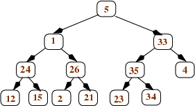
It is easiest to understand the heapify operation in terms of the tree represented by the array, but it can actually be performed on the array itself. The idea is to work bottom-up in the tree, turning each subtree into a heap. We will illustrate the process using the tree shown below.
We start with the nodes that are parents of leaves. For each such node n, we compare n's value to the values in its children, and swap n's value with its larger child if necessary. After doing this, each node that is the parent of leaves is now the root of a (small) heap. Here's what happens to the tree shown above after we heapify all nodes that are parents of leaves:
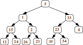
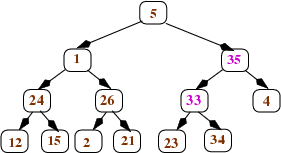
Then we continue to work our way up the tree: After applying heapify to all nodes at depth d, we apply it to the nodes at depth d-1. Each such node n will have 2 children, and those children will be the roots of heaps. If n's value is greater than the values in its children, we're done: n is the root of a heap. If not, we swap n's value with its larger child, and continue to swap down as needed (just like we do for the removeMax operation after moving the last leaf to the root). This happens in our example tree when we aply heapify to the right child of the root (the node containing the value 33). We swap that value with the larger child (35) to get this tree (with the changed values in pink):
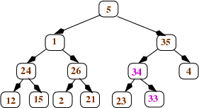
And then we swap the 33 with its larger child (34):
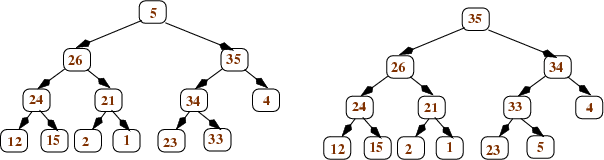
Once we apply heapify to the root, we're done: the whole tree is a heap. Here are the trees that result from applying heapify first to the left child of the root and then to the root itself:
It should be clear that, in the worst case, each heapify operation takes time proportional to the height of the node to which it is applied. Therefore, the total time for turning an array of size N into a heap is the sum of the heights of all nodes:
total time = sum from i=1 to N of height(i)
where the i's are the nodes of the tree. This is equivalent to
sum from k=1 to log N of k*(N/2k)
Here, k is height(i) and (N/2k) is the maximum number of nodes at that height. For example, k is 1 for all leaves and there are at most N/2 leaves; k is log N for the root and there is at most 1 root. We can convert as follows:
= sum from k=1 to log N of k*(N/2k) = N * sum from k=1 to log N of (k/2k)
The final sum is bounded by a constant, so the whole thing is just O(N)! One way to get some intuition for why it is just O(N) is to consider that most nodes have small heights: half of the nodes (the leaves) have height 1; another half of the remaining nodes have height 2, and so on.
The total time for heap sort is still O(N log N), because it takes time O(N log N) to perform the N removeMax operations, but using heapify does speed up the sort somewhat.
So far, the sorts we have been considering have all been comparison sorts (which can never have a worst-case running time less than O(N log N)). We will now consider a sort that is not a comparison sort: radix sort. Radix sort is useful when the values to be sorted are fairly short sequences of Comparable values. For example, radix sort can be used to sort numbers (sequences of digits) or strings (sequences of characters). The time for radix sort is O((N + range) * len)), where
For example, sorting 100 4-digit integers would take time (100 + 10) * 4, and sorting 1000 10-character words (where each word contains only lower-case letters) would take time (1000 + 26) * 10.
There are a number of variations on radix sort. The one presented here uses an auxiliary array of queues and works by processing each sequence right-to-left (least significant "digit" to most significant). On each pass, the values are taken from the original array and stored in a queue in the auxiliary array based on the value of the current "digit". Then the queues are dequeued back into the original array, ready for the next pass.
On the first pass, the position in the auxiliary array is determined by looking at the rightmost "digit" and each sequence is put into the queue in that position of the array. For example, suppose we want to sort the following original array:
We would use an auxiliary array of size 10 (since each digit can range in value from 0 to 9). After the first pass, the array of queues would look like this (where the array is shown vertically, indicated by position numbers, and the fronts of the queues are to the left):
0:
1: 111, 391
2: 132
3: 543, 123
4: 104
5: 355, 285, 535
6:
7: 327
8:
9:
Then we would make one pass through the auxiliary array, putting all values back into the original array:
On the next pass, the position in the auxiliary array is determined by looking at the second-to-right "digit":
0: 104
1: 111
2: 123, 327
3: 132, 535
4: 543
5: 355
6:
7:
8: 285
9: 391
Values are again put back into the original array:
and then the final pass chooses array position based on the leftmost digit (since we are sorting sequences of digits of length 3):
0:
1: 104, 111, 123, 132
2: 285
3: 327, 355, 391
4:
5: 535, 543
6:
7:
8:
9:
Putting the values back, we have a sorted array:
Each pass of radix sort takes time O(N) to put the values being sorted into the correct queue, and time O(N + range) to put the values back into the original array. The number of passes is equal to the number of "digits" in each value, so the total time is O((N + range) * len). This is often better than an O(N log N) sort. For example, log2 1,000,000 is about 20, so if we want to sort 1,000,000 numbers in the range 0 to 1,000,000, we have
Selection Sort:
Insertion Sort:
Merge Sort:
Quick Sort:
Heap Sort:
Radix Sort: