Pointer Analysis

Susan Horwitz
University of Wisconsin

Contents

Overview

For most dataflow-analysis problems, the definition of the dataflow function for each statement (each CFG node) depends on what locations are defined and/or used by that statement. In the absence of aliasing, the def/use sets can be determined simply by looking at the statement. For example, for the statement x = y + z, we can see that x is defined, while y and z are used. (Call statements are an exception -- as we've seen, even in a language without aliasing, interprocedural analysis is need to determine what variables might be defined and/or used by a procedure call.)

If the only source of aliasing is reference parameters, we can use the GMOD/GREF computations discussed in the paper Fast Interprocedural Alias Analysis by Cooper and Kennedy (or in the on-line notes on interprocedural analysis) to determine, for each reference parameter, to what other reference parameters and to what globals it might be aliased, and for each global, to what reference parameters it might be aliased. However, pointers introduce another kind of aliasing that cannot be handled by the usual GMOD/GREF computation.

For example, consider the following code:

 x = 0;
 *p = 1;
 print(x);
In order to solve dataflow problems like constant propagation, reaching definitions, or live variables, we need to know what variables might be modified by the statement *p = 1, which in turn requires knowing what locations p might point to at line 2. To determine that information we need to use some kind of pointer analysis.

The goal of pointer analysis is to determine safe points-to information for each CFG node; i.e., to determine for each CFG node, for each variable v, what locations v might be pointing to. Since we are interested in locations that might be pointed to, safe means a superset of the actual information; i.e., we want to err on the side of including too many locations in a points-to set, not too few.

We will consider several ways to do pointer analysis for a C-like language, including single-procedure analysis using Kildall's lattice model, and several flow-insensitive, whole-program analyses. We will start by ignoring complicating language aspects like heap-allocated storage, arrays, structures, and casting, but we'll talk about them at the end.

Flow-Sensitive Pointer Analysis

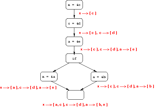
To do intraprocedural pointer analysis using our usual lattice model and iterative algorithm, we need to determine the following: One standard way to define the lattice of dataflow facts is using mappings from variables to sets of possibly pointed-to locations. Since we're ignoring heap storage for now, the possibly pointed-to locations will also be variables. And since we want the set of possibly pointed-to locations, the meet operation needs to include a location in a variable's points-to set whenever the location is in that set in either operand; i.e., the two sets of possibly pointed-to locations must be unioned together. An example CFG and its dataflow facts is given below.


TEST YOURSELF #1

For each of the following kinds of statements, say which variables' points-to sets would be changed by the corresponding dataflow function, and how they would be changed.


Unfortunately, given no information about other procedures we would have to use very conservative dataflow functions for calls, and very conservative initial dataflow facts (for the entry nodes of the procedures). In particular, for a call we would have to update the points-to sets for all of the following: We would have to add all of the above variables to the points-to sets of all of the above variables. And for the entry node of a procedure other than main we would have to assume that all globals and formals might point to all globals and formals.

Note that at the start of a procedure, a global or formal may also point (directly or transitively) to a local variable of some other procedure. However, this is not relevant for most uses of the results of pointer analysis. For example, when doing live-variable analysis on this sequence of statements:

we only care whether p may point to x or to y (to determine whether x is live immediately after the first assignment and whether y is live immediately after the second assignment); we don't care whether p may point to a local of another procedure.

We can get better results using the supergraph rather than using safe dataflow functions for calls and enter nodes. Another option is to use less precise but also less expensive flow-insensitive algorithms for pointer analysis, discussed below.

Flow-Insensitive Pointer Analysis

Flow-insensitive analysis ignores the flow of control in a program, and simply computes one dataflow fact for the whole program. One way to think about the goal of flow-insensitive analysis is that you model a program whose CFG has n nodes as a single node with n self-loop edges. Each edge has one of the dataflow functions from the nodes of the original CFG. Then you apply Kildall's iterative algorithm. Of course, the idea is to find a more efficient way to get the same result.

In general, even perfect flow-insensitive analysis provides very conservative results. It is not likely to be useful for dataflow problems like constant propagation, live variables, or reaching definitions. However, it seems to be useful in practice for pointer analysis.

Below we discuss four flow-insensitive pointer-analysis techniques. They vary in terms of their precision (how close they come to computing the same results as the ideal version defined above that uses a single-node CFG) and their worst-case runtimes:

  1. Andersen (1994)
  2. Steensgaard (1996)
  3. Shapiro (1997)
  4. Das (2000)
All four techniques assume that the program being analyzed has been normalized so that there is no more than one pointer dereference per statement. For example, the statements would be replaced by

Andersen's Analysis

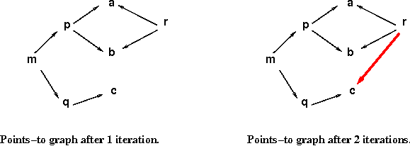
The way to understand Andersen's analysis is that it processes each statements in the program (in arbitrary order), building a points-to graph, until there is no change. (In a points-to graph, the edge ab means that a may point to b.) For example, suppose we're given the following set of statements: After one pass over this set of statements we would have the points-to graph shown below on the left, and after two iterations we would have the (final) graph shown below on the right (with the new edge added during the second iteration shown in red).

The actual algorithm is more efficient than this. Instead of building a points-to graph directly, it builds and manipulates a constraint structure, and only re-evaluates the effects of a statement that might cause a change in the points-to information. Nevertheless, the worst-case time for Andersen's algorithm is cubic (O(N3)) in the size of the program (assuming that the number of variables is linear in the size of the program).

To get some intuition on that N3 worst-case time, note that the most expensive assignment statements to process are those that involve a level of indirection; i.e., x = *y or *y = x. In both cases, we need to look at everything in the points-to set of y, and then everything in each of those points-to sets. in the worst case, y could point to all N variables in the program, and each of those could itself point to all N variables. Thus, processing the statement could involve O(N2) work. Since there are O(N) statements in the program, the total amount of work could be as much as O(N3).


TEST YOURSELF #2

Draw the points-to graph that would be produced by Andersen's analysis for the following set of statements:


Steensgaard's Analysis

Steensgaard's analysis also involves building a points-to graph, but his approach only requires that the set of statements be processed once (in any order), and the time required to process a statement is also reduced. To accomplish this, the algorithm merges some nodes, and limits the out-degree of any node to one (i.e., no node, merged or unmerged, has more than one outgoing edge).

To process one assignment statement the algorithm performs the following steps:

  1. Find the node n that represents the variable or variables being assigned to.
  2. Find the node m that represents the value being assigned.
  3. If node n already has an outgoing edge (to a node p != m) then merge m and p; otherwise, add an edge n → m.
  4. If m and p were merged then also merge the nodes that they point to if needed, and so on.
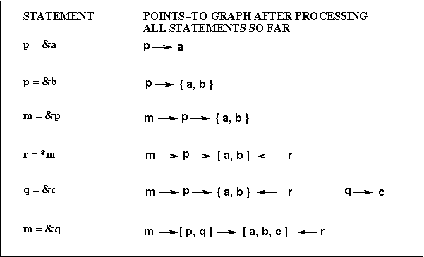
Below is the same example code that was used to illustrate Andersen's algorithm, and the points-to graphs that would be built by Steensgaard algorithm assuming that the statements are processed in the order given.

Note: If steps 1 and/or 2 involve a node that isn't in the graph yet, then a dummy node is added. This is illustrated by the example below.

Processing one statement can cause multiple nodes to be merged, but the total number of merges can be no more than the number of variables. Merging nodes and finding a representative node are done using Tarjan's union-find algorithm, which has worst-case time proportional to inverse Ackermann, which is essentially constant. Therefore, the whole algorithm is linear in the size of the program.


TEST YOURSELF #3

Draw the points-to graph that would be produced by Steensgaard's analysis for the following set of statements:


Shapiro's Analysis

Shapiro's analysis actually involves two (related) algorithms. The insight behind the first algorithm is that we can build a points-to graph (like Andersen and Steensgaard), but (unlike those two algorithms) we can allow a user-specified amount of out-degree. This makes the algorithm "tunable": if we restrict the out-degree to 1, we get Steensgaard's algorithm; if we allow outdegree n (where n is the number of variables in the program), we get Andersen's algorithm.

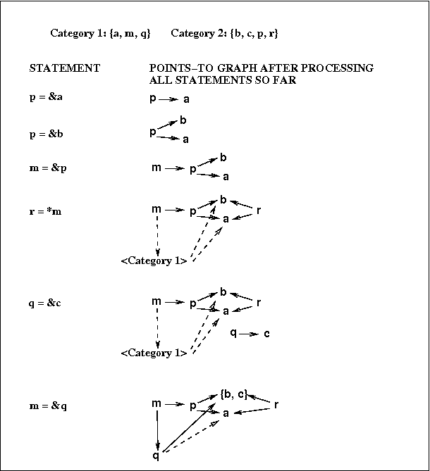
Given value k (the amount of out-degree to allow), Shapiro's first algorithm divides the variables in the program into k "categories". It then processes each statement in the program once, updating the points-to graph to reflect the effect of the statement. When the points-to graph is updated to make a variable x point to both v1 and v2, the nodes for v1 and v2 are merged iff v1 and v2 are in the same category. As in Steensgaard's approach, if an update to the points-to graph involves a node that isn't in the graph yet, one or more dummy nodes are added. A dummy node has "tentative" outgoing edges (one for each category). The tentative edge for category c gets turned into a regular points-to edges if the dummy node gets filled in, and its points-to set for category c also gets filled in.

This technique is illustrated below, using our running example.

In this example, the results of Shapiro's points-to analysis are less precise than Andersen's (because the points-to facts pc and qb, are included) but more precise than Steensgaard's (because the points-to-fact qa is not included).

Note that the choice of categories is important: if instead of the categories used in the above example we had used { a, c, q, m } and { b, p, r }, the result would have been closer to the result using Andersen's analysis; and if we had used { a, b, c } and { p, q, r, m }, the result would have been the same as Steensgaard's analysis.

However, although different choices of categories can lead to different results, all of those results are safe, This leads to an interesting observation: If the points-to sets computed using different categories are all safe (are all over approximations, e.g., the sets may be too large but are never too small) then the intersections of the results are also safe. This leads to the second version of Shapiro's points-to analysis:


TEST YOURSELF #4

Analyze the code given below using one category (to get the same results as Steensgaard's algorithm); using two categories: {a, b} and {c, d}; and using four categories (to get the same results as Andersen's algorithm). Then try using the two categories: {a, c} and {b, d}, and intersect the results with the results you got using the previous two categories.


An important question is how to assign variables to categories, and how to choose T (the number of times to run the original algorithm with different categories). One interesting answer investigated by Shapiro was to let the user choose the number of categories, k (between 2 and N, where N is the number of variables), then to use T = ceiling(logk(N)). This way, the categories can be chosen so that for every pair of variables there is at least one run for which they are in different categories. To do this:

For example, suppose we have four variables (a to d) and k=2. Then the number of runs will be log2(4) = 2. Here are the variables with their numbers: On the first run, the categories will be {a,b} and {c,d}, while on the second run they will be {a,c} and {b,d}.

The worst-case time for the first version of Shapiro's algorithm is O(k2 N), where N is the size of the program and k is the number of categories. As for Andersen's algorithm, the worst case for processing a single assignment statement is for a statement of the form x = *y or *y = x. This requires examining the targets of all edges out of y in the points-to graph, and then all edges out of those nodes. There are at most k edges out of any node, so the total number of edges that might need to be followed is k2. Each of the N statements in the program is processed once, so the total worst-case time is no more than O(k2 N).

For the second version, the total time is O(T k 2 N). To guarantee that there is at least one run that "separates" every pair of variables, we get O(logk k2 N).

Das's Analysis

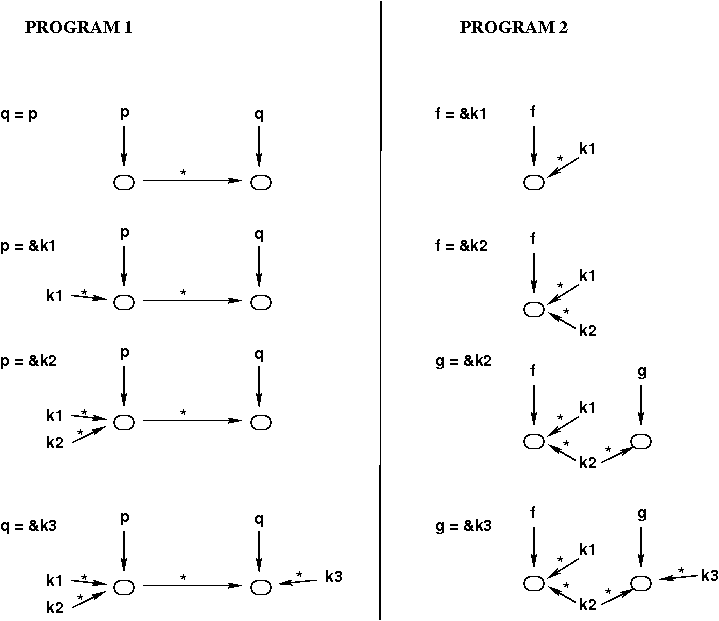
Das's algorithm is based on the observation (made by doing studies of C programs) that in C code, most pointers arise because the address of a variable is passed as a parameter. This is done either to simulate call-by-reference (i.e., so that the procedure can modify that parameter), or for efficiency (e.g., when the parameter is a struct or an array). This observation is important because the use of pointer parameters can cause Steensgaard's algorithm to lose precision when a pointer parameter is passed on from one procedure to another, or when two different procedures are called with the same pointer parameter. For example, consider the two programs shown below. For each program, the actual code is shown on the left, and the equivalent set of assignment statements is shown on the right. Here are the points-to graphs that would be built using Andersen's analysis and using Steensgaard's analysis:
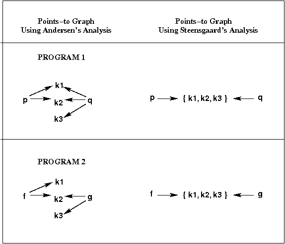
The loss of precision for Program 1 (the inclusion of the "extra" fact pk3), occurs when processing the assignment q = p. The way Steensgaard handles a "copy assignment" like that is to merge the points-to sets of the left- and right-hand side variables; i.e., to treat the assignment as symmetric. Das handles q = p differently: instead of merging points-to sets, he introduces what he calls a flow edge into the points-to graph from the node that represents p's points-to set to the node that represents q's points-to set. (If those nodes don't exist, empty dummy nodes are added.) This flow edge means that all of the addresses in the points-to set of p are also in the set of q. In fact, flow edges are introduced when processing all assignment statements, including ones of the form v1 = &v2. As in Steensgaard's algorithm, each node in the points-to graph has only a single outgoing "points-to" edge, but it can have any number of outgoing flow edges.

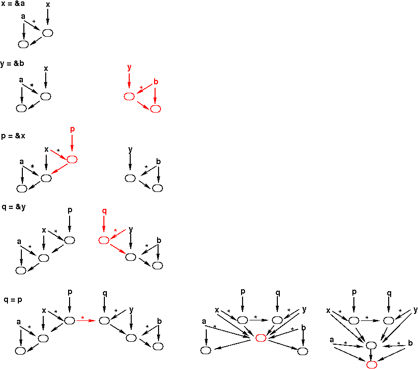
Below are the sequences of assignments for example Programs 1 and 2 again, and the corresponding sequences of points-to graphs built by Das's algorithm. The points-to graphs shown are actually slightly simplified; we will see the missing parts below. In the graphs, points-to edges are shown as plain arrows, and flow edges are shown as arrows with stars above them.

Like Steensgaard, Das processes each assignment in the program just once, building a points-to graph with both points-to and flow edges. After the graph is built, sets of variables must be propagated forward along the flow edges to form the final points-to sets. The results of this propagation step for the two final points-to graphs shown above are shown below, along with the final points-to sets for each variable.

The simplification in the above points-to graphs has to do with the fact that Das's algorithm is similar to Steensgaard's in that it does merge some points-to sets. In particular, whenever a flow edge n1 *→ n2 is added, all points-to sets "below" n1 and n2 are merged. In order for this to work, whenever a flow edge n1 *→ n2 is added to the graph, outgoing points-to edges (to dummy nodes) are also added if they don't already exist. Below is an example that illustrates that, as well as illustrating the merging of points-to sets performed by Das's algorithm. The merging occurs after the last assignment (q = p). In the figure below, this is illustrated using three points-to graphs to illustrate (left-to-right)

  1. adding the flow edge that puts everything in p's points-to set into q's points-to set;
  2. merging the points-to sets below those of p and q;
  3. merging the points-to successors of the nodes that were just merged.
In each points-to graph, the new nodes and edges are shown in red.

It is worth noting that because Das's algorithm only merges nodes below a flow edge, it maintains precision for "top-level" pointers; i.e., pointers that are not themselves pointed to.

TEST YOURSELF #5

Draw the points-to graph and the final points-to sets that would be computed using Das's algorithm for the code below (that we used previously to illustrate the other flow-insensitive pointer analyses). Compare the final points-to sets with those computed by Andersen's algorithm.


Efficiency of Das's Algorithm

Das's algorithm works in two phases: building the points-to graph and propagating points-to sets. The first phase processes each assignment statement just once. The total number of nodes in the points-to graph is proportional to the number of assignments. Each node has exactly one outgoing points-to edge, and processing each assignment adds at most one flow edge (so the total number of edges is also proportional to the number of assignments). Therefore, the space used by phase 1 is linear in the program size. Processing an assignment "lhs = rhs" requires following a constant number of points-to edges, adding a flow edge, and possibly merging some nodes. Although more than one node may be merged as the result of processing one assignment, the total number of merges is bounded by the number of nodes in the graph (i.e., by the number of assignments). Tarjan's fast union/find algorithm is used so that each merge is constant time, and each find (to find the target of a points-to edge that points to a merged node) is proportional to inverse Ackermann, which is essentially linear. Thus, the total time for phase 1 is essentially linear in the size of the program.

The propagation step takes time proportional to the sum of the sizes of the final points-to sets. In the worst case, this is O(N2), where N is the number of variables. However, in practice (see Experimental Results below), the time appears to be linear.

Experimental Results

Das did some experiments to compare his algorithm with those of Andersen and Steensgaard. He found that