- link ID,
- link length (in ft),
- valid period (the time span during which the link is current in the database),
- from-reference-site, and
- to-reference-site.
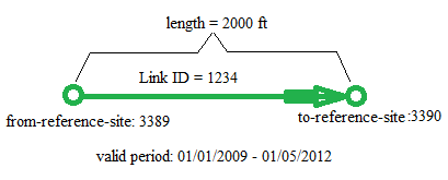
Figure 1 A typical Link object.
Each tuple (row) in the DT_RDWY_LINK table of WisTransportal STN database is loaded into the memory as a Link object (hereafter called a link for short) in the program. A link has the following properties (as shown in Figure 1):
|
Figure 1 A typical Link object. |
Additionally, in the second step, all crashes occurred on the same link will form a list and be added to that link.
Each tuple (row) in a crash table of WisTransportal is loaded into the memory as a Crash object (hereafter referred to as a crash). Only crashes within a user-specified analysis period are loaded. A crash has the following properties (as shown in Figure 2):
|
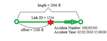 Figure 2 A typical Crash object. |
Crashes are not only loaded in a global list, but also added to the crash list of its containing link. So each link will have a list of crashes that happened in it. This list can be empty if there was not crash happening on this link during the user-specified analysis period.
A STS route is a a sequence of connected links connecting one reference site (RS) to another. By saying connected links, no enforcement is made on following the directions of links. Two links are treated as connected if their from-reference-sites are the same, their to-reference-sites are the same, or one's from-reference-site is the other's to-reference-site. Since no direction is enforced, a STS route is different from some traditional notion of route. The reason why direction is not concerned for now is that only the route length will be used in future calculation. Although no direction is used, link distinction is enforced. In other words, a link cannot appear more than once in a STS route. Also, a STS route can be 0 ft long if its corresponding start RS and end RS are identical. Figure 3 shows some examples of STS routes. Each STS route has the following properties:
|
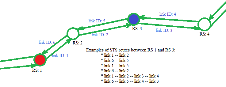 Figure 3 Illustration of STS routes. |
|||||||||||||||||||||||||||||||||||||||||||||||||
This step establishes a matrix of STS routes. The conceptual image of the matrix is illustrated in Figure 4. Each cell(i,j) contains a list of STS routes from RS_i to RS_j. There can be many STS routes from RS_i to RS_j, but only some of them are included in cell(i,j). The conditions for a STS route to be included are:
To save computing time and memory space, not all cells are calculated or stored. First, cell(i,j) is calculated only when RS_i is the from-reference-site or to-reference-site of a link that contains at least one crash. Second, cell(i,j) is only stored when it contains at least one STS route that satisfies the above two conditions. |
|
The following sub steps are performed on each link with at least one crash. For each of such links, we call it a base link.
A candidate link is defined as a link any of whose crashes might be within the distance filter from any of the crashes on the base link. A candidate link is identified in the following way: Assume the from- and to- reference-sites of the base link (B) are RS_bi and RS_bj. Given a link L, with from- and to- reference-sites being RS_li and RS_lj, L is a candidate link of B iff cell(bi,li), cell(bi,lj), cell(bj,li), and cell(bj,lj) have been calculated and stored in the STS route matrix during Step 3.
For each crash prim in base link B and each crash scnd in a candidate link L, we determine whether scnd is a potential secondary crash of prim in two stages: