1 Fictitious point |
9 Real points |
1 Fictitious point |
Suppose that there is a bug on a small beam. This bug hops a specific distance at specific time intervals. The directions of the hops are random, but are only in the lateral direction of the beam and are with equal probability to the left and right. There are only a certain number of hops on the beam. There is a depiction of this below.
We would like to know how many hops the bug might take before it falls off when it starts at any point. For example, it seems clear that if the bug starts in the middle of the bar it will take longer to fall off than if it starts next to an end. We can solve for the average number of hops it takes to walk off the edge for each starting point.
The equation for the average time to fall off is derived as follows: consider any given starting point, say, point k, and a particular path that the bug takes. The bug can go either to the left or the right with probability of one-half. Notice that once the bug is at the neighboring point, say k+1, the bug's future is the same as a bug that had started at that point. Thus, the time to fall off from point k in that case is one more than the time it takes to fall off as measured from point k+1. The same is true for the case where the bug went to k-1 instead of k+1. Thus, on average, the time it takes to fall off from point k is one more than the average time it takes to fall off from points k-1 and k+1. This gives us the following equation:

In other words, at each starting point, the average number of steps it takes (for a bug that is at that point) to fall off the edge of the bar is the average of the surrounding points plus the one step it took the bug to go to that position.
Important note: This is called mathematical modeling and is a very important aspect of engineering research. A physical phenomenon, a bug hopping on a bar, is translated into a mathematical description that allows us to compute numerical estimates of the process.
This formula works for points in the middle of the bar; what about points at the ends? A convenient way to handle the points at the ends of the bar is to add fictitious points beyond the bar. At these fictitious points the bug is already off the bar, therefore the number of steps to fall off the bar is zero and the equation for any fictitious point k is

In MATLAB, all vector and matrix indexes start with 1, so the first point (the fictitious point on the left) is 1 and the first point on the bar is numbered 2. So, the equation for point 1 (the fictitious point) is

And the equation for the average number of steps it takes to fall off starting from point 2 is

In this equation we don't have to be concerned that point 1 is fictitious and point 3 is an actual point. All the actual points have the same general equation and all the fictitious points have the same general equation. Without the fictitious points we would have to check whether an actual point is at the end or not, and an end point would have a different equation than a point that is not at an end. This is a complication that having fictitious points avoids.
Important note: Many engineering problems use ideas similar to those used here. Rather than bugs hopping around, engineers are interested in heat conduction, finite element stress analysis, neutron transport, chemical reactant diffusion, etc. The basic modeling process as a linear system is similar and the numerical trick of creating fictitious points to ease the numerical solution algorithm is similar.
Problem 1: Model the problem as a linear system in matrix form. (Do parts a - c on paper)
For each position, write a linear equation that computes the number of steps on average it takes a bug starting at that position to fall off the bar.
Tip: Number each position on the figure 1 through n, pick a variable name, T, and write out the equation for each starting position, T1 through Tn.
Reorder the terms in each equation so that each equation is in general form.
General form has the unknown terms on the left and the constants on the right of the equals sign. Be careful to write your equations so that all unknown terms "line up" with the corresponding unknown terms of the other equations.
Write the system as a single matrix equation.
Put the coefficients of the unknowns in a matrix and show the multiplication of that matrix with a column vector of the unknown variables, T1 through Tn, and set that equal to a column vector of the constants or known values.
SHOW YOUR EQUATIONS TO A LAB LEADER
Create a new script. Inside the script, add code to create the coefficient matrix and assign it to the name A.
The matrix A is a matrix of the coefficients of the unknown terms (Tk).
These commands can get you started. Note that putting each row of the matrix on a separate line improves readability and makes it easier to spot typos. Also note that if you put each row on a separate line when you are defining a matrix (as you are here), you don't need to end each line with ... (dot,dot,dot) to continue the statement on the next line.
A = [1 0 0 0 0 0 0 0 0 0 0;
-.5 1 -.5 0 0 0 0 0 0 0 0;
and so on ... until the last row
0 0 0 0 0 0 0 0 0 0 1];
Enter the data vector (right hand side column of the system) as a column vector named b.
b =
Use MATLAB's backslash operator to solve for the unknowns T.
T = A \ b
Don't forget to run your script. Do your results make sense (e.g., are all the values in T non-negative)?
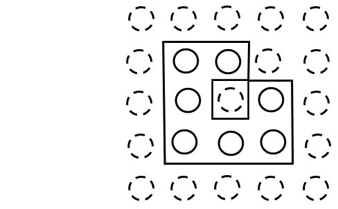
Problem 2: ... but, there are holes in the bar
Now create a linear system for the bar (below) which has a hole in it. The hole looks like a fictitious point in the middle area of the bar. Remember that the equation for a fictitious point is Tk=0. You need to revise the equation to account for the hole in the linear system.
You may have noticed that if the bar has holes in it, then the problem decomposes into separate problems, one for each section. However, we don't need to solve it as two problems, we just need to modify the equations and solve the new system. In the next section we will consider two-dimensional problems with holes, and these one-dimensional problems with holes are a good warm-up for the two-dimensional problems.
Problem 3: ... and he asks the bartender for a plate
Let's take this problem to two dimensions. There is a bug on a plate and it can hop north, south, east, or west. The average number of steps is still determined in the same way: it is the average of the points around it, plus one step to get to the next position. Here is the equation for a point p

where n, s, e, and w refer to the surrounding points to the north, south, east and west of point p. We have included a diagram to help you get started.
Create a system of linear equations that will solve for every point on the plate.
First, number the points from 1 to 25 on the diagram. Then determine the equations for each point, including the fictitious points.
SHOW YOUR EQUATIONS FOR PLATE POSITIONS 6, 7, 12, 13, 18, 19 TO A LAB LEADER
Enter the coefficient matrix. (Hint: the matrix will have one unknown for each position on the plate. You should see a pattern for the off-diagonal elements).
Try using the identity matrix function, A = eye(25,25), to get the coefficient matrix started.
One way you can create the coefficient matrix is to write the commands in a script that can be saved, edited, and re-executed as needed. After using the eye function, you need to set other values in just the rows that correspond to positions on the plate. Use commands similar to the following: A(2,[1,3])=-1/2 (which sets the values at columns 1 and 3 of row 2 of matrix A to the value -1/2).
Enter the right hand side column data vector. To make entering easier, remember that you can use built-in MATLAB functions like zeros() and ones() which can be useful for creating large matrices and vectors.
Solve the linear system.
Display the 25 solution values in the same organization as the plate (i.e., a 5×5 grid of corresponding values instead of a single list of 25 values).
SHOW YOUR SOLUTION IN THE 5×5 GRID FORMAT TO A LAB LEADER
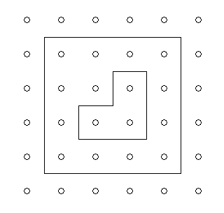
Problem 4: ... but, there are holes in the plate, too!
Now let's consider a plate with holes:
Modify your linear system from problem 3 to account for the holes and solve it. As in part 3.e, display the solution values in the same organization as the plate.
Here's another plate with holes for you to try (note that this plate is 4×4):
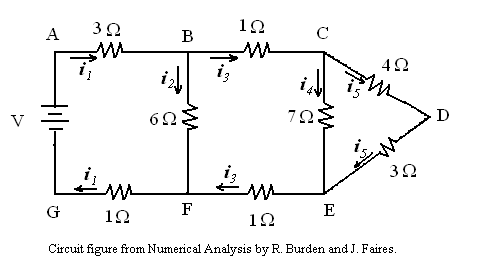
A simple DC circuit is given below:
Given the voltages and resistances in the branches, we wish to compute the currents. Resistances are given in Ohms (Ω), there is an applied voltage (V), and arrows indicate the direction of positive current. The basic principles for DC circuits are expressed as Kirchhoff's Laws. These two laws give the set of linear equations that need to be solved to obtain the currents (labelled with i's in the diagram).
Kirchhoff's First Law: (node equations) The sum of the current flowing into a node must be equal to the sum of the current flowing out of the node.
This leads to the following equations for the nodes:
Note that the equations for nodes A, D, G, E, and F are redundant and can be thrown out.
Kirchhoff's Second Law: (loop equations) The sum of the products of the resistance (Ohms) times the current around a cycle will be zero.
This leads to the following equations for loops:
Note that the loop equation for loop 4 provides redundant information and thus finding every possible cycle is not necessary. Simply find non-redundant cycles.
You will need to assign a value for the voltage to actually solve the linear system. Try V=6 and V=9.