Lambda Calculus (Part I)


Contents


Overview

Lambda calculus is a model of computation, invented by Church in the early 1930's. Lambda calculus and Turing machines are equivalent, in the sense that any function that can be defined using one can be defined using the other. Here are some points of comparison:

Lambda Calculus Turing Machine
Forms the basis for functional languages (LISP, Scheme, ML). Forms the basis for imperative languages (Pascal, ADA, C).
We write a lambda expression for each function. Input and output are also lambda expressions. Design a new machine to compute each function. Input and output are written on tape.

A Simple Example

Here's an example of a simple lambda expression that defines the "plus one" function:

(Note that this example does not illustrate the pure lambda calculus, because it uses the + operator, which is not part of the pure lambda calculus; however, this example is easier to understand than a pure lambda calculus example.)

This example defines a function of one argument, whose formal parameter is named 'x'. The function body is: "x+1". Note that the function has no name (i.e., it is an anonymous function). To compute with this function, we need to apply it to an argument; for example:

In this example, λx.x+1 is the function, and 3 is the argument; the entire thing is itself a lambda expression.

Computation involves re-writing:

For now, think of rewriting as replacing all occurrences of the formal parameter 'x' in the function with the argument (and then, for a non-pure lambda expression that includes operators like plus, applying those operators). We'll get to a more precise definition later.

Lambda Calculus Syntax

The syntax of (pure) lambda expressions is defined as follows:

  1. A variable is a lambda expression (we will use single, lower-case letters for variables).
  2. If M and N are lambda expressions, then so are each of the following:
    1. (M)
    2. λid.M
    3. MN
That's all!

Rule 2(a) just says that we can put parenthesis around anything. Rule 2(b) defines what we call an abstraction: a function whose formal parameter is id, and whose body is M. Rule 2(c) defines what we call an application: we apply one lambda expression to another (M is applied to N).

Note that the pure lambda calculus excludes constants, types, and primitive operators (e.g. +, *, ...). Note also that (by convention) application is left associative: ABC means (AB)C not A(BC), and application has higher precedence than abstraction: λx.AB means λx.(AB), not (λx.A)B

We can express the rules given above that define the language of lambda expressions using a context-free grammar:
exp ID
| ( exp )
| λ ID . exp // abstraction
| exp exp // application

As mentioned above, computing with lambda expressions involves rewriting; for each application, we replace all occurrences of the formal parameter (a variable) in the function body with the value of the actual parameter (a lambda expression). It is easier to understand if we use the abstract-syntax tree of a lambda expression instead of just the text. Here's our simple example application again:

And here's the abstract-syntax tree (where λ is the abstraction operator, and apply is the application operator):
        apply
        /   \
       λ     3
      / \
     x   +
        / \
       x   1
We rewrite the abstract syntax tree by finding applications of functions to arguments, and for each, replacing the formal parameter with the argument in the function body. To do this, we must find an apply node whose left child is a lambda node, since only lambda nodes represent functions. There is only one apply node in our example; the argument is 3, the function is λx.x+1; the formal parameter is x, and the function body is x+1. Here's the rewriting step:
        apply      =>      +
        /   \             / \
       λ     3           3   1
      / \
     x   +
        / \
       x   1
Here's an example with two applications: The first lambda expression defines the "plus-one" function. The argument to that function is itself an application, which applies the "plus-two" function to the value 3. Here's the abstract-syntax tree and one way to do the rewriting (choosing to rewrite the rightmost application first):
        apply         =>   apply     =>  apply   =>  +  =>  6
       /     \             /   \         /   \      / \
      λ       apply       λ     +       λ     5    5   1
     / \       /  \      / \   / \     / \
    x   +     λ    3    x   + 3   2   x   +
       / \   / \           / \           / \
      x   1 y   +         x   1         x   1
               / \
              y   2
In general, different strategies for choosing which application to rewrite first can have different ramifications. That issue is discussed below.


TEST YOURSELF #1

Do the rewriting again, this time choosing the other application first.

solution


Note that the result of rewriting a non-pure lambda expression can be a constant (as in the examples above), but the result can also be a lambda expression: a variable, or an abstraction, or an application. For a pure lambda expression, the result of rewriting will always itself be a lambda expression. Here are some more examples:

  1. (λf.λx.fx)λy.y+1
    The first lambda expression defines a function whose argument, f, is also a function, and whose body, λx.fx is yet another function (one that takes an argument x, and applies f to it). Below are the abstract-syntax tree and the rewriting; you might want to try to draw them yourself before looking.
            apply      =>   λ        =>    λ        λx.x+1
           /     \         / \            / \
          λ       λ       x  apply       x   +    
         / \     / \         /   \          / \
        f   λ   y   +       λ     x        x   1
           / \     / \     / \
          x  apply y  1   y   +
             /  \            / \
            f    x          y   1
    
    Note that the result of the rewriting is a function. Also note that in this example, although there are initially two "apply" nodes, only one of them has a lambda node as its left child, so there is only one rewrite that can be done initially.

  2. (λx.λy.x)(λz.z)
    In this example, the first lambda takes one argument, x, and returns a function that ignores its own argument (y), simply returning x. In this example, the value supplied for x is itself a function.
    
               apply            λ         λy.λz.z
              /     \          / \
             λ       λ    =>  y   λ      
            / \     / \          / \
           x   λ   z   z        z   z
              / \
             y   x


TEST YOURSELF #2

Draw the abstract-syntax tree for the lambda expression given below, then do the rewriting steps.

solution


Problems with the naive rewriting rule

Recall that the imprecise definition of rewriting an application (λx.M)N is "M with all occurrences of x replaced by N". However, there are two problems with this definition.

Problem #1: We don't, in general, want to replace all occurrences of x. To see why, consider the following (non-pure) lambda expression:

This expression should reduce to 6; the inner expression: takes one argument, the value 3, and adds 1, producing 4. The outer expression is now: i.e., it takes one argument, the value 2, and adds 4, producing 6.

However, if we rewrite the outer application first, using the naive rewriting rule, here's what happens:

We get the wrong answer (5 instead of 6), because we replaced the occurrence of x in the inner expression with the value supplied as the parameter for the outer expression.

Problem #2: Consider the (pure) lambda expression

This is like one of the examples given above, except that this time we apply λx.λy.x to two arguments (y and z) instead of just one argument (λz.z). When applied to two arguments, the expression λx.λy.x should simply return the first argument, so in this case the result of rewriting should be y. However, if we use the naive rewriting rule, replacing all occurrences of the formal parameter x with the argument y, we get: and now if we rewrite that expression we get i.e., we got the second argument instead of the first one! This example illustrates what is called the "capture" or "name clash" problem.

To understand how to fix the first problem illustrated above, we first need to understand scoping, which involves the following terminology:

Intuitively, in lambda-expression M, variable x is bound if, in the abstract-syntax tree, x is in the subtree of a lambda with left child x:

                λ
               / \
              x  /\
                /  \
               /    \
              /..x...\
                 |
                 this x is bound
Here is a precise definition of free and bound variables:
  1. In the expression x, variable x is free (no variable is bound).
  2. In the expression λx.M, every x in M is bound; every variable other than x that is free in M is free in λx.M; every variable that is bound in M is bound in λx.M.
  3. In the expression MN:
    1. The free variables of MN are the union of two sets: the free variables of M, and the free variables of N.
    2. The bound variables of MN are also the union of two sets: the bound variables of M and the bound variables of N.
Note that a variable may occur more than once in some lambda expression; some occurrences may be free and some may be bound, so the variable itself is both free and bound in the expression, but each individual occurrence is either free or bound (not both). For example, the free variables of the following lambda expression are {y,x} and the bound variables are {y}:
            (λx.y)(λy.yx)
                |     ||
                |     |free
               free   |
                    bound
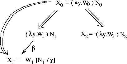
To solve problem #1 above, given lambda expression instead of replacing all occurrences of x in M with N, we replace all occurrences of x that are free in M with N. For example:
                       +----- M ---------+
                       |                 |
                   (λx. x + ((λx.x + 1)3)) 2
                        |        |
                        |        |
                       free    bound
                       in M    in M

                     => 2 + ((λx.x + 1)3)
The issue behind problem #2 is that a variable y that is free in the original argument to a lambda expression becomes bound after rewriting (using that argument to replace all instances of the formal parameter), because it is put into the scope of a lambda with a formal that happens also to be named y:
    ((λx.λy.x)y)z
              |
              |
              free, but gets bound after application 

To solve problem #2, we use a technique called alpha-reduction. The basic idea is that formal parameter names are unimportant; so rename them as needed to avoid capture. Alpha-reduction is used to modify expressions of the form "λx.M". It renames all the occurrences of x that are free in M to some other variable z that does not occur in M (and then λx is changed to λz). For example, consider λx.λy.x+y (this is of the form λx.M). Variable z is not in M, so we can rename x to z; i.e.,

Here is pseudo code for alpha reduction.

Note: Another way to handle problem #2 is to use what's called de Bruijn notation, which uses integers instead of identifiers. That possibility is explored in the first homework assignment.

Beta-reduction

We are finally ready to give the precise definition of rewriting:

We use the following notation for beta-reduction;

The left-hand side ((λx.M)N) is called the redex. The right-hand side (M[N/x]) is called the contractum and the notation means M with all free occurrences of x replaced with N in a way that avoids capture. We say that (λx.M)N beta-reduces to M with N substituted for x. And here is pseudo code for substitution.

To illustrate beta-reduction, consider the previous example of problem #2. Here are the beta-reduction steps:
        ((λx.λy.x)y)z
                ->  ((λy.x)[y/x])z   // substitute y for x in the body of "λy.x"
                ->  ((λy'.x)[y/x])z  // after alpha reduction
                ->  (λy'.y)z         // first beta-reduction complete!
                ->  y[z/y']          // substitute z for y' in "y"
                ->  y                // second beta-reduction complete!
Note that the term "beta-reduction" is perhaps misleading, since doing beta-reduction does not always produce a smaller lambda expression. In fact, a beta-reduction can: the length of a lambda expression. Below are some examples. In the first example, the result of the beta-reduction is the same as the input (so the size doesn't change); in the second example, the lambda expression gets longer and longer; and in the third example, the result first gets longer, and then gets shorter.

Normal Form

As discussed above, computing with lambda expressions involves rewriting them using beta-reduction. There is another operation, beta expansion that we can also use. By definition, lambda expression e1 beta-expands to e2 iff e2 beta-reduces to e1. So for example, the expression

beta-expands to each of the following:

A computation is finished when there are no more redexes (no more applications of a function to an argument). We say that a lambda expression without redexes is in normal form, and that a lambda expression has a normal form iff there is some sequence of beta-reductions and/or expansions that leads to a normal form.

This leads to some interesting questions about normal form:

  1. Q: Does every lambda expression have a normal form ?
    A: No, e.g.: (λz.zz)(λz.zz). Note that this should not be surprising, since lambda calculus is equivalent to Turing machines, and we know that a Turing machine may fail to halt (similarly, a program may go into an infinite loop or an infinite recursion).

  2. Q: If a lambda expression does have a normal form, can we get there using only beta-reductions, or might we need to use beta-expansions, too?
    A: Beta-reductions are good enough (this is a corollary to the Church-Rosser theorem, coming up soon!)

  3. Q: If a lambda expression does have a normal form, do all choices of reduction sequences get there?
    A: No. Consider the following lambda expression:
      (λx.λy.y)((λz.zz)(λz.zz))
    This lambda expression contains two redexes: the first is the whole expression (the application of (λx.λy.y) to its argument); the second is the argument itself: ((λz.zz)(λz.zz)). The second redex is the one we used above to illustrate a lambda expression with no normal form; each time you beta-reduce it, you get the same expression back. Clearly, if we keep choosing that redex to reduce we're never going to find a normal form for the whole expression. However, if we reduce the first redex we get: λy.y, which is in normal form. Therefore, the sequence of choices that we make can determine whether or not we get to a normal form.

  4. Q: Is there a strategy for choosing beta-reductions that is guaranteed to result in a normal form if one exists?
    A: Yes! It is called leftmost-outermost or normal-order-reduction (NOR), and we'll define it below.

Normal-Order and Applicative-Order Reduction

Definition: An outermost redex is a redex that is not contained inside another one. (Similarly, an innermost redex is one that has no redexes inside it.) In terms of the abstract-syntax tree, an "apply" node represents an outermost redex iff

  1. it represents a redex (its left child is a lambda), and
  2. it has no ancestor "apply" node in the tree that also represents a redex.

For example:

                            apply  <-- not a redex
                           /     \
an outermost redex --> apply      apply <-- another outermost redex
                      /    \      /    \
                     λ     ...   λ      apply  <-- redex, but not outermost
                    / \         / \     /   \     
                  ... ...      ... ... λ    ...

To do a normal-order reduction, always choose the leftmost of the outermost redexes (that's why normal-order reduction is also called leftmost-outermost reduction).

Normal-order reduction is like call-by-name parameter passing, where you evaluate an actual parameter only when the corresponding formal is used. If the formal is not used, then you save the work of evaluating the actual. The leftmost outermost redex cannot be part of an argument to another redex; i.e., reducing it is like executing the function body, rather than evaluating an actual parameter. If it is a function that ignores its argument, then reducing that redex can make other redexes (those that define the argument) "go away"; however, reducing an argument will never make the function "go away". This is the intuition that explains why normal-order reduction will get you to a normal form if one exists, even when other sequences of reductions will not.


TEST YOURSELF #3

Fill in the incomplete abstract-syntax tree given above (to illustrate "outermost" redexes) so that the resulting lambda expression has a normal form and the only way to get there is by choosing the leftmost outermost redex (instead of some other redex) at some point in the reduction.

solution


You may be wondering whether it is a good idea always to use normal-order reduction (NOR). Unfortunately, the answer is no; the problem is that NOR can be very inefficient. The same issue arises with call-by-name parameter passing: if there are many uses of a formal parameter in a function, and you evaluate the corresponding actual each time the formal is used, and evaluating the actual is expensive, then you would have been better off simply evaluating the actual once. This leads to the definition of another useful evaluation order: leftmost innermost or applicative-order reduction (AOR). For AOR we always choose the leftmost of the innermost redexes. AOR corresponds to call-by-value parameter passing: all arguments are evaluated (once) before the function is called (or, in terms of lambda expressions, the arguments are reduced before applying the function). The advantage of AOR is efficiency: if the formal parameter appears many times in the body of the function, then NOR will require that the actual parameter be reduced many times while AOR will only require that it be reduced once. The disadvantage is that AOR may fail to terminate on a lambda expression that has a normal form.

It is worth noting that, for programming languages, there is a solution called call-by-need parameter passing that provides the best of both worlds. Call-by-need is like call-by-name in that an actual parameter is only evaluated when the corresponding formal is used; however, the difference is that when using call-by-need, the result of the evaluation is saved and is then reused for each subsequent use of the formal. In the absence of side-effects (that cause different evaluations of the actual to produce different values), call-by-name and call-by-need are equivalent in terms of the values computed (though call-by-need may be more efficient).


TEST YOURSELF #4

Define a lambda expression that can be reduced to normal form using either NOR or AOR, but for which AOR is more efficient.

solution


The Church-Rosser Theorem

Now it's time for our first theorem: The Church-Rosser Theorem. First, we need one new definition:

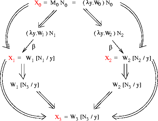
Theorem: if (X0 red X1) and (X0 red X2), then there is an X3 such that: (X1 red X3) and (X2 red X3). Pictorially:


                       X0
                     /    \ 
                    /      \
                   /        \
                  v          v
                 X1          X2
                  \          /
                   \        /
                    \      / 
                     \    /
                      v  v
                       X3
where the arrows represent sequences of zero or more alpha- and/or beta-reductions.

Corollaries: if X has normal form Y then

  1. X reduces to Y using only alpha and/or beta reductions (no expansions are needed), and
  2. Y is unique (up to alpha-reduction); i.e., X has no other normal form.

First we'll assume that the theorem is true, and prove the two corollaries; then we'll prove the theorem. To make things a bit simpler, we'll assume that we're using DeBruijn notation; i.e., no alpha-reduction is needed.

Proof of Corollary 1

To prove Corollary 1, note that "X has normal form Y" means that we can get from X to Y using some sequence of interleaved beta-reductions and beta-expansions. Pictorially we have something like this:

                            ^
                           /
              ^           /
             /    \      /    ......  \
            /      \    /              \
         X          v                   \
                                         v
                                         Y
where the upward-pointing arrows represent a sequence of beta-expansions, and the downward-pointing arrows represent a sequence of beta-reductions. Note that we cannot end with an expansion, since Y is in normal form.

We will prove Corollary 1 by induction on the number of changes of direction in getting from X to Y.

Base cases

  1. Zero changes of direction. Since, as noted above, we cannot end with an expansion, the picture must be:
               X
                \
                 \
                  v
                   Y
    
    i.e., we got from X to Y using zero or more beta-reductions, so we're done.

  2. 1 change of direction; i.e. the picture is:
    
                  W
                ^    \
               /      \      
              /        \   
             /          v
           X            Y 
    
    i.e., we first use some beta-expansions to get from X to some lambda expression W, then use some beta-reductions to get from W to Y. Because every beta-expansion is the inverse of a beta-reduction, this means that we can get from W to X (as well as from W to Y) using a sequence of beta-reductions; i.e., we have the following picture:
                            W
                          /   \
                         /     \
                        /       \
                       v         v
                       X         Y
    
    The Church-Rosser Theorem guarantees that there's a Z such that both X and Y reduce to Z:
    
                 W     
               /   \          
              /     \     
             v       v
            X         Y        
             \       / 
              \     /  
               v   v
                 Z
    
    Since Y is (by assumption) in normal form, it must be that Y = Z, and our picture really looks like this:
    
                 W     
               /   \          
              /    |
             v     |
            X      |
             \     |
              \   /
               v v
                Y
    
    which means that X reduces to Y without any expansions.

    Now we're ready for the induction step:

    Induction Hypothesis: If X has normal form Y, and we can get from X to Y using a sequence of beta-expansions and reductions that involve n changes of direction (for n >= 1), then we can get from X to Y using only beta-reductions.

    Now we must show that (given the induction hypothesis) Corollary 1 holds for n+1 changes of direction.

    Here's a picture of an X and a Y such that n+1 changes of direction are needed to get from X to Y:

    
              W
             ^  \           ^  \          ^  \
            /    \         /    \        /    \
           /      \       /      \      /
          /        v     /        v    /       v
         X           ...           ...          Y
    
       <--1 change --> <-- n changes of direction -->
    
    Note that there is some lambda expression W (shown in the picture above) such that:
    1. We can get from X to W using a series of beta-expansions, and
    2. we can get from W to Y using beta expansions and reductions, with n changes of direction.
    By the induction hypothesis, point 2 above means that we can get from W to Y using only beta reductions:
    
               W
                \
                 \
                  v
                  Y
    
    Combining this with point 1 we have:
    
                 W
               ^   \ 
              /     \
             /       \ 
            /         v
           X          Y
    
    In other words, we can get from X to W using only beta-expansions, and from W to Y using only beta-reductions. Using the same reasoning that we used above to prove the second base case, we conclude that we can get from X to Y using only beta-reductions.

    Proof of Corollary 2

    Recall that Corollary 2 says that if lambda-term X has normal form Y then Y is unique (up to alpha-reduction); i.e., X has no other normal form. We can prove that by contradiction: Assume that, in contradiction to the Corollary, Y and Z are two different normal forms of X. By Corollary 1, X reduces to both Y and Z:

                                  X
                                /   \
                               /     \
                              /       \
                             v         v
                             Y         Z
    
    By the Church-Rosser Theorem, this means there is W, such that:
    
                    X
                  /  \
                 /    \
                v      v
               Y        Z
                \      /
                 \    /
                  v  v
                    W
    
    However, since by assumption Y and Z are already in normal form, there are no reductions to be done; thus, Y = W = Z, and X does not have two distinct normal forms.

    Proof of the Church-Rosser Theorem

    Recall that the theorem is:

      if (X0 red X1) and (X0 red X2), then there is an X3 such that: (X1 red X3) and (X2 red X3).

    Where "red" means "zero or more beta-reductions" (since we're assuming de Bruijn notation, and thus ignoring alph-reductions).

    We'd like to prove the theorem by "filling in the diamond" from X0 to X3; i.e., by showing that something like the following situation must exist:

                              X0                 
                            /   \                
                          W1     Z1              
                         /  \  /   \
                       W2     A     X2
                      /   \  /  \  /
                    X1     B     C
                      \   /  \  /
                        D     E
                          \  /
                            F  = X3
    
    In other words, we'd like to show that for every lambda term, if you can take two different "steps" (can do two different beta-reductions) to terms A and B, then you can come back to a common term C by doing one beta-reduction from A, and one from B. If we could show that, then we'd have the desired X3 by construction as shown in the picture above.

    Unfortunately, this idea doesn't quite work; i.e., it is not true in general that we can get to common term C in just one step from A and one step from B. Below is an example that illustrates this, using * to mean a redex that reduces to y.

    
            X0 = (λx.xx)(*)
                /          \
               /            \
            (**)             (λx.xx)y
              \                  /
               \                /
                \              /
             (y*) or (*y)     /
                       \     /
                        \   /
                         (yy)
    
    Note that there are two redexes in the initial term X0: * itself, and the one in which * is the argument to a lambda-term. So we can take two different "steps" from X0, arriving either at (**) or at (λx.xx)y. While we can come back to a common term, (yy), from both of those, it requires two steps from (**).

    So to prove the Church-Rosser Theorem, we need a new definition:

    Definition (the diamond property): A relation ~~> on terms has the diamond property iff

      ( X0 ~~> X1) and ( X0 ~~> X2) implies there is an X3 such that ( X1 ~~> X3 ) and ( X2 ~~> X3 )

    Note:

    1. The Church-Rosser Theorem says that the relation beta-reduce* has the diamond property (i.e., if X beta-reduces to both A and B in zero or more steps, then both A and B beta-reduce to C in zero or more steps).
    2. The previous example showed that single beta reduction does not have the diamond property (just because X beta-reduces to both A and B in one step does not mean that both A and B beta-reduce to C in one step).

    The three tasks

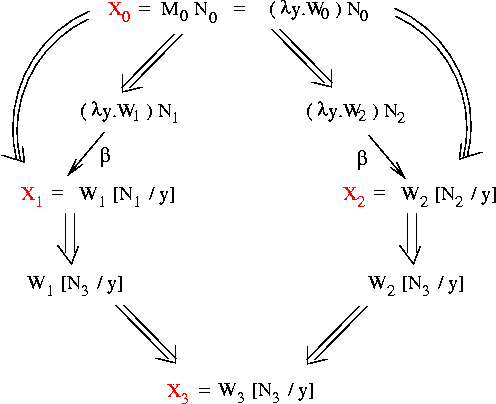
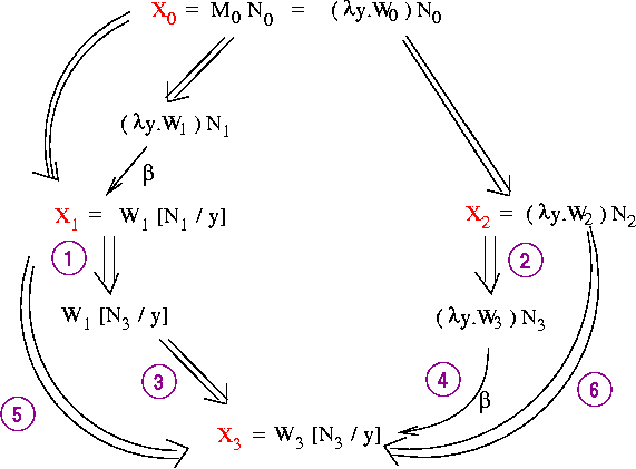
    To prove the Church-Rosser Theorem we will perform the following 3 tasks:

    1. Define a new relation called a walk (written ⇒).
    2. Prove that X beta-reduce* Y iff X ⇒* Y
    3. Prove that ⇒ has the diamond property.

    Finally, we'll prove that ⇒* (a sequence of zero or more walks) has the diamond property, and we'll use that to "fill in the diamond" and thus to prove the Church-Rosser Theorem.

    Task 1

    Definition (walk): A walk is a sequence of zero or more beta-reductions restricted as follows:

      If the ith reduction in the sequence reduces a redex r, then no later reduction in the sequence can reduce an instance of a redex that was inside r; i.e., reductions must be done bottom-up in the abstract-syntax tree.

    Here are some examples (again, * means a redex that reduces to y):

          (λx.xx)(*)      
             | 
             |
             v
          (λx.xx)y
             |
             | 
             v
             yy
    
    This entire reduction sequence (2 beta-reductions) is a walk because the inner redex is reduced first. Here's what the reductions look like using the abstract-syntax tree:
    
             apply                     apply                  apply
             /     \                   /    \                 /   \
           λ        *                 λ      y               y     y 
         /   \               -->    /  \          -->      
       x    apply                  x   apply              
            /   \                      /    \
          x      x                    x      x
    
    However, consider this sequence of beta-reductions (starting with the same initial term), first showing the lambda terms, then the abstract-syntax trees:
           (λx.xx)(*)
               |
               | 
               v
             (**)
               |
               |
               v
             (y*)
               |
               |
               v
             (yy)


            apply           apply           apply           apply
           /    \           /   \           /    \          /    \
          λ      *         *     *         y      *        y     y
        /  \        -->              -->             -->
       x   apply
           /   \
          x     x
    
                    ==>             =======================>
               this step is a       these two steps constitute a walk
               walk    
    
    Although as noted above, the first beta-reduction is a walk, and the second and third together are also a walk, the sequence of three reductions is not a walk because once the root "apply" is chosen to be reduced (which happens as the first reduction), no apply in the tree can be reduced as part of the same walk (so the reductions of the two "*" terms are illegal).

    Here are two important insights about walks:

    1. You can't always concatenate two walks and get a walk (i.e., walk is not a transitive relation).
    2. Two walks that reduce non-overlapping redexes can be concatenated to form a walk.

    NOTE: We've now accomplished task (1) toward proving the Church-Rosser Theorem.

    Task 2

    Task 2 involves proving that (X beta-reduce* Y) iff (X walk* Y).

    The => direction is trivial; we must show that every sequence of zero or more beta-reductions is also a sequence of walks. Since each individual beta-reduction is a walk, we just let the sequence of walks be exactly the sequence of beta-reductions.

    The <= direction is easy, too. Every walk is a sequence of zero or beta-reductions. So every sequence of walks is a concatenation of sequences of beta-reductions, which is itself a sequence of beta-reductions.

    Task 3

    For task 3 of our proof of the Church-Rosser Theorem we must prove a lemma that says that the walk relation has the diamond property. We'll call that CRT Lemma 2, because to do that proof we first need another lemma:

    CRT Lemma 1 (the walk relation is preserved when free variables are replaced by terms): if (X ⇒ Y) then (X[P/x] ⇒ Y[P/x])

    (Note: X ⇒ Y means "X walk Y", and X[P/x] means X with the free occurrences of x replaced by P without capture.)

    We won't give a formal proof of the Lemma; instead we'll convince ourselves by considering what happens to the free occurrences of x in X when X ⇒ Y (remember that X ⇒ Y means zero or more of the redexes in X are reduced bottom-up):

    1. A free occurrence of x can be in the body of a function that is a part of a redex that is reduced as part of X ⇒ Y. In this case, the occurrence of x continues to be free after reduction. So if that occurrence of x is replaced by P before the reduction we get the same thing as if it is replaced by P after the reduction.

    2. A free occurrence of x can be in an argument that is a part of a redex that is reduced as part of X ⇒ Y. There are two subcases:

      (i) If x is "ignored" by the function part of the redex, (i.e., the function body does not include any occurrences of its formal parameter) then there will be no occurrences of x after the reduction, so replacing occurrences of x with P after the reduction is an empty operation; similarly, if we replace x with P before the reduction there will be NO occurrences of P after the reduction. Thus, it doesn't matter if we do the substitution before or after.

      (ii) If x is not ignored, then there will be one or more occurrences of x after the reduction; if the x's are replaced with P's before the reduction then there will be the same number of P's after the reduction. Note that these occurrences of x cannot be themselves reduced when X ⇒ Y, because the x's are variables, not applications. So again we get the same thing by doing the substitution before or after the reduction.


    TEST YOURSELF #5

    Show that CRT Lemma 1 is not iff; i.e., find an example X, Y, and P such that (X[P/x] ⇒ Y[P/x]) but it is not true that (X ⇒ Y).

    solution


    Now we can prove CRT Lemma 2.

    CRT Lemma 2 ( ⇒ has the diamond property): if (X0 ⇒ X1) and (X0 ⇒ X2) then there is an X3 such that (X1 ⇒ X3) and (X2 ⇒ X3).

    Pictorially, Lemma 2 says that given X0, X1, and X2 with the following relationship (where the diagonal lines mean a walk):

    
                        X0
                     //   \\
                   //      \\
                  v          v    
                 X1          X2
    
    we're guaranteed to have an X3 with the following relationship to X1 and X2:
    
                        X0
                     //   \\
                   //      \\
                  v          v    
                 X1          X2
                   \\       //
                    \\     //
                      v   v
                       X3
    
    We will prove this by structural induction: induction on the height of the abstract-syntax tree for X0.

    Base case: X0 is a variable (i.e., the height of the tree = 1).

    In this case, to get from X0 to X1 or from X0 to X2 must require zero reductions (since a variable has no redexes). So X0 = X1 = X2, and the X3 we're looking for is the same thing, too: X0 = X3.

    Inductive Step: Assume that CRT Lemma 2 holds for all lambda terms X0 with abstract-syntax tree of height less than or equal to n; show that it holds for all terms of height n+1. Note that there are two ways to get a lambda term of height n+1:

    1. By creating a term of the form λx.M0 (i.e., an abstraction), where M0 is a term of height n, or
    2. By creating a term of the form M0 N0 (i.e., an application) where either M0 or N0 is of height n, and the other is of height <= n.

    Case 1: X0 is of the form λx.M0

    Case 2: X0 is of the form M0 N0

    The final proof

    Now that we've accomplished our three tasks, it remains to show that ⇒* has the diamond property, and to use that fact to prove the original theorem.

    In fact, it can be shown that given any relation ~~> that has the diamond property, ~~>* also has the diamond property. That is left as an exercise; we will give an informal argument here.

    We want to show that for given a lambda term X0 such that X0 ⇒* X1, and X0 ⇒* X2, there exists an X3 such that X1 ⇒* X3, and X2 ⇒* X3. Pictorially, we have:

    
                            X0
                         //    \\ 
                         v      v
                        W1      Z1
                        //      \\
                        v        v
                       ...      ...
                       //        \\
                       v          v
                      X1          X2
    
    and we want to show:
    
                            X0
                         //    \\ 
                         v      v
                        W1      Z1
                        //      \\
                        v        v
                       ...      ...
                       //        \\
                       v          v
                      X1          X2
                      \\          //
                       v          v
                      ...       ...
                        \\      // 
                         \\    //
                          v   v
                            X3
    
    Since we know that each individual walk has the diamond property, we can "fill in the diamonds" as shown below, creating a sequence of walks from both X1 to X2, and X2 to X3:
    
    
                            X0
                         //    \\
                        W1      Z1
                       // \\  //  \\
                      W2     A      Z2
                     //\\  // \\  //  \\
                    W3   B       C      Z3
                   //\\//\\    // \\  // \\
                  ... ... ... ... ... ... ...
                  //\\//\\    // \\  // \\ //\\
                  X1                          X2
                   \\ ...                    //
                  ... ... ... ... ... ... ...
                           \\  //
                             X3
    

    Now for the final proof of the Theorem. Recall that we need to show that if (X0 red X1) and (X2 red X2), then there is an X3 such that (X1 red X3) and (X2 red X3). Task 2 showed that (X0 red X1) implies that (X0 ⇒* X1), and similarly for X2; in other words, we can get from X0 to either X1 or X2 using a sequence of walks. Since ⇒* has the diamond property, this means that we can also get from either X1 or X2 to X3 using a sequence of walks, and we have:

      (X0 ⇒* X1) and (X0 ⇒* X2) and (X1 ⇒* X3) and (X2 ⇒* X2).

    Using the result of task 2 again, we note that a sequence of walks is also a sequence of beta reductions, so (X1 ⇒* X3) implies (X1 red X3), and similarly for X2, and so we're done!