| Lung Function (Y) | Smoking Status (A) |
|---|---|
| 0.940 | Never |
| 0.918 | Never |
| 0.808 | Daily |
| 0.838 | Never |
Causal Inference: Basic Concepts and Randomized Experiments
Concepts Covered Today
- Association versus causation
- Defining causal quantities with counterfactual/potential outcomes
- Connection to missing data
- Identification of the average treatment effect in a completely randomized experiment
- Covariate balance
Does daily smoking cause a decrease in lung function?
Data: 2009-2010 National Health and Nutrition Examination Survey (NHANES).
- Treatment (\(A\)): Daily smoker (\(A = 1\)) vs. never smoker (\(A = 0\))
- Outcome (\(Y\)): ratio of forced expiratory volume in one second over forced vital capacity. \(Y \geq\) 0.8 is good lung function!
- Sample size is \(n=\) 2360.
Association of Smoking and Lung Function
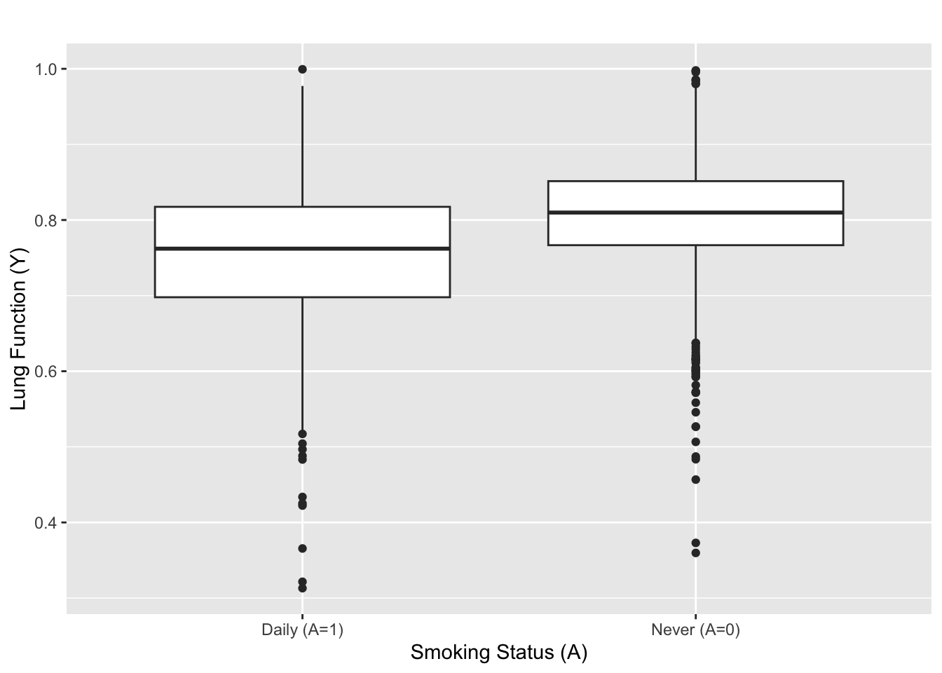
- \(\overline{Y}_{\rm daily (A = 1) }=\) 0.75 and \(\overline{Y}_{\rm never (A = 0)}=\) 0.81.
- \(t\)-stat \(=\) -11.8, two-sided p value: \(\ll 10^{-16}\)
Daily smoking is strongly associated with 0.06 reduction in lung function.
But, is the strong association evidence for causality?
Definition of Association
Association: \(A\) is associated with \(Y\) if \(A\) is informative about \(Y\)
- If you smoke daily \((A = 1)\), then it’s likely that your lungs aren’t functioning well (\(Y\)).
- If smoking status doesn’t provide any information about lung function, \(A\) is not associated with \(Y\).
Formally, \(A\) is associated with \(Y\) if \(\mathbb{P}(Y | A) \neq \mathbb{P}(Y)\).
Some parameters that measure association:
- Population difference in means: \(\mathbb{E}[Y | A=1] - \mathbb{E}[Y | A=0]\)
- Population covariance: \({\rm cov}(A,Y) = \mathbb{E}[ (A - \mathbb{E}[A])(Y - \mathbb{E}[Y])]\)
Estimators/tests that measure association:
- Sample difference in means, regression, etc.
- Two-sample t-tests, Wilcoxon signed-rank test, etc.
Defining Causation: Parallel Universe Analogy

Suppose John’s lung functions are different between the two universes.
- The difference in lung functions can only be attributed to the difference in smoking status.
- Why? All variables (except smoking status) are the same between the two parallel universes.
Key Point: comparing outcomes between parallel universes enable us to say any difference in the outcome must be due to a difference in the treatment status.
This provides a basis for defining a causal effect of \(A\) on \(Y\).
Counterfactual/Potential Outcomes
Notation for outcomes in parallel universes:
- \(Y(1)\): counterfactual/potential lung function if you smoked (i.e. parallel world where you smoked)
- \(Y(0)\): counterfactual/potential lung function if you didn’t smoke (i.e. parallel world where you didn’t smoke)
Similar to the observed data table, we can create counterfactual/potential outcomes data table.
| \(Y(1)\) | \(Y(0)\) | |
|---|---|---|
| John | 0.5 | 0.9 |
| Sally | 0.8 | 0.8 |
| Kate | 0.9 | 0.6 |
| Jason | 0.6 | 0.9 |
For pedagogy, we’ll assume that all data tables are an i.i.d. sample from some population (i.e. \(Y_i(1), Y_i(0) \overset{\text{i.i.d.}}{\sim} \mathbb{P}\{Y(1),Y(0)\}\)).
Note on super-population versus finite population
Similar to the observed data \((Y,A)\), you can think of the counterfactual data table as an i.i.d. from some population distribution of \(Y(1),Y(0)\) (i.e. \(Y_i(1), Y_i(0) \overset{\text{i.i.d.}}{\sim} \mathbb{P}\{Y(1),Y(0)\}\))
- This is often referred to as the super-population framework.
- Expectations are defined with respect to the population distribution (i.e. \(\mathbb{E}[Y(1)] = \int y \mathbb{P}(Y(1) = y)dy\))
- The population distribution is fixed and the sampling generates the source of randomness (i.e. i.i.d. draws from \(\mathbb{P}\{Y(1),Y(0)\}\), perhaps \(\mathbb{P}\{Y(1),Y(0)\}\) is jointly Normal?)
- For asymptotic analysis, \(\mathbb{P}\{Y(1),Y(0)\}\) is usually fixed (i.e. \(\mathbb{P}\{Y(1),Y(0)\}\) does not vary with sample size \(n\)). In high dimensional regimes, \(\mathbb{P}\{Y(1),Y(0)\}\) will vary with \(n\).
Or, you can think of \(n=4\) as the entire population.
- This is often referred to as the finite population/randomization inference or design-based framework.
- Expectations are defined with respect to the table above (i.e. \(\mathbb{E}[Y(1)] = (0.5+0.8+0.9+0.6)/4 =0.7\) )
- The counterfactual data table is the population and the treatment assignment (i.e. which counterfactual universe you get to see; see below) generates the randomness and the observed sample.
- For asymptotic analysis, both the population (i.e. the counterfactual data table) and the sample changes with \(n\). In some vague sense, asymptotic analysis under the finite sample framework is inherently high dimensional.
Finally, you can think of data above as a simple random sample of size \(n\) from a finite population of size \(0 < n < N < \infty\).
The latter two frameworks are uncommon in typical statistics courses, especially the second one. However, it’s very popular among some circles of causal inference folks (e.g. Rubin, Rosenbaum and their students). The appendix of Erich Leo Lehmann (2006), Rosenbaum (2002b), and Li and Ding (2017) provide a list of technical tools to conduct this type of inference.
There has been a long debate about which the “right” framework for inference. My understanding is that it’s now (i.e. Apr. 2024) a matter of personal taste. Also, as Paul Rosenbaum puts it:
In most cases, their disagreement is entirely without technical consequence: the same procedures are used, and the same conclusions are reached…Whatever Fisher and Neyman may have thought, in Lehmann’s text they work together. (Page 40, Rosenbaum (2002b))
The textbook that Paul is referring to is (now) Erich L. Lehmann and Romano (2006). Note that this quote touches on another debate in the literature in finite-sample inference, which is what is the correct null hypothesis to test. In general, it’s good to be aware of the differences between the frameworks and, as Lehmann did (see full quote), use the strengths of each different frameworks. For some interesting discussions on this topic, see Robins (2002), Rosenbaum (2002a), Chapter 2.4.5 of Rosenbaum (2002b), and Abadie et al. (2020). For other papers in this area, see Splawa-Neyman, Dabrowska, and Speed (1990), Freedman and Lane (1983), Freedman (2008), and Lin (2013).
Causal Estimands
| \(Y(1)\) | \(Y(0)\) | |
|---|---|---|
| John | 0.5 | 0.9 |
| Sally | 0.8 | 0.8 |
| Kate | 0.9 | 0.6 |
| Jason | 0.6 | 0.9 |
Some quantities/parameters from the counterfactual outcomes:
- \(Y_{\rm John}(1) - Y_{\rm John}(0) = -0.4\): Causal effect of John smoking versus not smoking (i.e. individual treatment effect)
- \(\mathbb{E}[Y(1)]\): Average of counterfactual outcomes when everyone is a daily smoker.
- \(\mathbb{E}[Y(1) - Y(0)]\): Difference in the average counterfactual outcomes when everyone is smoking versus when everyone is not smoking (i.e. average treatment effect, ATE)
A causal estimand/parameter is a function of the counterfactual outcomes.
Counterfactual Data Versus Observed Data
Table 1: Comparison of tables.
| \(Y(1)\) | \(Y(0)\) | |
|---|---|---|
| John | 0.5 | 0.9 |
| Sally | 0.8 | 0.8 |
| Kate | 0.9 | 0.6 |
| Jason | 0.6 | 0.9 |
| \(Y\) | \(A\) | |
|---|---|---|
| John | 0.9 | 0 |
| Sally | 0.8 | 1 |
| Kate | 0.6 | 0 |
| Jason | 0.6 | 1 |
For both, we can define parameters (i.e. \(\mathbb{E}[Y]\) or \(\mathbb{E}[Y(1)]\)) and take i.i.d. samples from their respective populations to learn them.
- \(Y_i(1), Y_i(0) \overset{\text{i.i.d.}}{\sim} \mathbb{P}\{Y(1), Y(0)\}\) and \(\mathbb{P}\) is Uniform, etc.
If we can observe the counterfactual table, we can run your favorite statistical methods and estimate/test causal estimands.
The Main Problem of Causal Inference
If we can observe all counterfactual outcomes, causal inference reduces to doing usual statistical analysis with \(Y(0),Y(1)\).
But, in many cases, we don’t get to observe all counterfactual outcomes.
A key goal in causal inference is to learn about the counterfactual outcomes \(Y(1), Y(0)\) from the observed data \((Y,A)\).
- How do we learn about causal parameters (e.g. \(\mathbb{E}[Y(1)]\)) from the observed data \((Y,A)\)
- What causal parameters are impossible to learn from the observed data?
Addressing this type of question is referred to as causal identification.
Causal Identification: SUTVA or Causal Consistency
First, let’s make the following assumption known as stable unit treatment value assumption (SUTVA) or causal consistency (Rubin (1980), page 4 of Hernán and Robins (2020)).
\[Y = AY(1) + (1-A) Y(0)\]
Equivalently,
\[Y = Y(A) \text{ or if } A=a, Y = Y(a)\]
The assumption states the observed outcome is one realizaton of the counterfactual outcomes.
- It also states that there are no multiple versions of treatment.
- It also states that there is no interference, a term coined by Cox (1958).
No Multiple Versions of Treatment
Daily smoking (i.e. \(A=1\)) can include different type of smokers
- Daily smoker who smokes one pack of cigarettes per day
- Daily smoker who smokes one cigarette per day
- Daily smoker who vapes per day
The current \(Y(1)\) does not distinguish outcomes between different types of smokers.
We can define counterfactual outcomes for all kinds of daily smokers, say \(Y(k)\) for \(k=1,\ldots,K\) type of daily smokers. But, if \(A=1\), which counterfactual outcome should this correspond to?
SUTVA eliminates these variations in the counterfactuals. Or, if \(Y(k)\) exists, it assumes that these variations \(Y(1) = Y(2) = \ldots =Y(K)\).
Implicitly, SUTVA forces you to define meaningful \(Y(a)\). Some authors restrict counterfactual outcomes to be based on well-defined interventions or “no causation without manipulation” (Holland (1986),Hernán and Taubman (2008),Cole and Frangakis (2009), VanderWeele (2009)).
Causal effect of race or gender
A healthy majority of people in causal inference argue that the counterfactual outcome of race and gender are ill-defined. For example, suppose we re interested in whether being a female causes lower income. We could define the counterfactual outcomes as
- \(Y(1)\): Jamie’s income when Jamie is female
- \(Y(0)\): Jamie’s income when Jamie is not female
Similarly, we are interested in whether being a black person causes lower income, we could define the counterfactual outcomes as
- \(Y(1)\): Jamie’s income when Jamie is black
- \(Y(0)\): Jamie’s income when Jamie is not black
But, if Jamie is a female, can there be a parallel universe where Jamie is a male? That is, is there a universe where everything else is the same (i.e. Jamie’s whole life experience up to 2024, education, environment, maybe Jamie gave birth to kids), but Jamie is now a male instead of a female?
Note that we can still measure the association of gender on income, for instance with a linear regression of income (i.e \(Y\)) on gender (i.e. \(A\)). This is a well-defined quantity.
There is an interesting set of papers on this topic: VanderWeele and Robinson (2014), Vandenbroucke, Broadbent, and Pearce (2016), Krieger and Davey Smith (2016), VanderWeele (2016). See Volume 45, Issue 6, 2016 issue of the International Journal of Epidemiology.
Some even take this example further and argue whether counterfactual outcomes are well-defined in the first place; see Dawid (2000) and a counterpoint in Sections 1.1, 2 and 3 of Robins and Greenland (2000).
No Interference
Suppose we want to study the causal effect of getting the measles vaccine on getting the measles. Let’s define the following counterfactual outcomes:
- \(Y(0)\): Jamie’s counterfactual measles status when Jamie is not vaccinated
- \(Y(1)\): Jamie’s counterfactual measles status when Jamie is vaccinated
Suppose Jamie has a sibling Alex and let’s entertain the possible values of Jamie’s \(Y(0)\) based on Alex’s vaccination status.
- Jamie’s counterfactual measles status when Alex is vaccinated.
- Jamie’s counterfactual measles status when Alexis not vaccinated.
The current \(Y(0)\) does not distinguish between the two counterfactual outcomes.
No Interference
We can again define counterfactual outcomes to incorporate this scenario, say \(Y(a,b)\) where \(a\) refers to Jamie’s vaccination status and \(b\) refers to Alex’s vaccination status.
SUTVA states that Jamie’s outcome only depends on Jamie’s vaccination status, not Alex’s vaccination status. Or, more precisely \(Y(a,b) = Y(a,b')\) for all \(a,b,b'\).
In some studies, the no interference assumption is not plausible (e.g. vaccine studies, peer effects in classrooms/neighborhoods, air pollutions). Rosenbaum (2007) has a nice set of examples of when the no interference assumption is not plausible.
There is a lot of ongoing work on this topic (Rosenbaum (2007),Hudgens and Halloran (2008), Tchetgen and VanderWeele (2012)). I am interested in in this area as well and let me know if you want to learn more.
Causal Identification and Missing Data
Once we assume SUTVA (i.e. \(Y= AY(1) + (1-A)Y(0)\)), causal identification can be seen as a problem in missing data.
| \(Y(1)\) | \(Y(0)\) | \(Y\) | \(A\) | |
|---|---|---|---|---|
| John | NA | 0.9 | 0.9 | 0 |
| Sally | 0.8 | NA | 0.8 | 1 |
| Kate | NA | 0.6 | 0.6 | 0 |
| Jason | 0.6 | NA | 0.6 | 1 |
Under SUTVA, we only see one of the two counterfactual outcomes based on \(A\).
- \(A\) serves as the “missingness” indicator where \(A=1\) implies \(Y(1)\) is observed and \(A=0\) implies \(Y(0)\) is observed.
- \(Y\) is the “observed” value.
- Being able to only observe one counterfactual outcome in the observed data is known as the ``fundamental problem of causal inference’’ (page 476 of Holland (1988)).
Assumption on Missingness Pattern
| \(Y(1)\) | \(Y(0)\) | \(Y\) | \(A\) | |
|---|---|---|---|---|
| John | NA | 0.9 | 0.9 | 0 |
| Sally | 0.8 | NA | 0.8 | 1 |
| Kate | NA | 0.6 | 0.6 | 0 |
| Jason | 0.6 | NA | 0.6 | 1. |
Suppose we are interested in learning the causal estimand \(\mathbb{E}[Y(1)]\) (i.e. the mean of the first column).
One approach would be to take the average of the “complete cases” (i.e. Sally’s 0.8 and Jason’s 0.6).
- Formally, we would use \(\mathbb{E}[Y | A=1]\), the mean of the observed outcome \(Y\) among \(A=1\).
- This approach is valid if the entries of the first column are missing completely at random (MCAR)
- In other words, the missingness indicator \(A\) flips a random coin per each individual and decides whether its \(Y(1)\) is missing or not.
This is essentially akin to a randomized experiment.
Formal Statement of MCAR
Formally, MCAR can be stated as \[A \perp Y(1) \text{ and } 0 < \mathbb{P}(A=1)\]
- \(A \perp Y(1)\) states that missingness is independent of \(Y(1)\)
- Missingness occurs completely at random in the rows of the first column, say by a flip of a random coin.
- Missingness doesn’t occur more frequently for higher values of \(Y(1)\); this would violate \(A \perp Y(1)\).
- \(0 < \mathbb{P}(A=1) <1\) states that you have a non-zero probability of observing some entries of the column \(Y(1)\)
- If \(\mathbb{P}(A=1) =0\), then all entries of the column \(Y(1)\) are missing and we can’t learn anything about its column mean.
Formal Proof of Causal Identification of \(\mathbb{E}[Y(1)]\)
Suppose SUTVA and MCAR hold:
- (A1): \(Y = A Y(1) + (1-A) Y(0)\)
- (A2): \(A \perp Y(1)\)
- (A3): \(0 < \mathbb{P}(A=1)\)
Then, we can identify the causal estimand \(\mathbb{E}[Y(1)]\) by writing it as the following function of the observed data \(\mathbb{E}[Y | A=1]\): \[\begin{align*} \mathbb{E}[Y | A=1] &= \mathbb{E}[AY(1) + (1-A)Y(0) | A=1] && \text{(A1)} \\ &= \mathbb{E}[Y(1)|A=1] && \text{Definition of conditional expectation} \\ &= \mathbb{E}[Y(1)] && \text{(A2)} \end{align*}\] (A3) is used to ensure that \(\mathbb{E}[Y | A=1]\) is a well-defined quantity.
Using a Mean-Independence Assumption for Identification
Technically speaking, to establish \(\mathbb{E}[Y(1)] = \mathbb{E}[Y | A=1]\), we only need \(\mathbb{E}[Y(1) | A=1] = \mathbb{E}[Y(1)]\) and \(0 < \mathbb{P}(A=1)\) instead of \(A \perp Y(1)\) and \(0 < \mathbb{P}(A=1)\); note that \(A \perp Y(1)\) is equivalent to \(\mathbb{P}(Y(1) | A=1) = \mathbb{P}(Y(1))\). In words, we only need \(A\) to be unrelated to \(Y(1)\) in expectation, not necessarily in the entire distribution.
Causal Identification of the ATE
In a similar vein, to identify the ATE \(\mathbb{E}[Y(1)-Y(0)]\), a natural approach would be to use \(\mathbb{E}[Y | A=1] - \mathbb{E}[Y | A=0]\), respectively.
This approach would be valid under the following variation of the MCAR assumption: \[A \perp Y(0),Y(1), \quad{} 0 < \mathbb{P}(A=1) < 1\]
- The first part states that the treatment \(A\) is independent of \(Y(1), Y(0)\). This is called exchangeability or ignorability in causal inference.
- \(0 < \mathbb{P}(A=1) <1\) states that there is a non-zero probability of observing some entries from the column \(Y(1)\) and from the column \(Y(0)\). This is called positivity or overlap in causal inference.
Why \(A \perp Y(1)\) is not equivalent to \(A \perp Y\)
Note that \(A \perp Y(1)\) (i.e. missingness indicator \(A\) for the \(Y(1)\) column is completely random) is not equivalent to \(A \perp Y\) (i.e. \(A\) is not associated with \(Y\)), with or without SUTVA.
- Without SUTVA, \(Y\) and \(Y(1)\) are completely different variables and thus, the two statements are generally not equivalent to each other. In other words, \(A \perp Y(1)\) makes an assumption about the counterfactual outcome whereas \(A \perp Y\) makes an assumption about the observed outcome.
- With SUTVA, \(Y = Y(1)\) only if \(A =1\) and thus, \(A \perp Y(1)\) does not necessarily imply that \(Y = AY(1) + (1-A)Y(0)\) is independent of \(A\). To put it differently, \(A \perp Y(1)\) only tells about the lack of relationship between the column of \(Y(1)\) and the column of \(A\). In contrast, \(A \perp Y\) tells me about the lack of relationship between the column \(Y\), which is a mix of \(Y(1)\) and \(Y(0)\) under SUTVA, and the column of \(A\).
Formal Proof of Causal Identification of the ATE
Suppose SUTVA and MCAR hold:
- (A1): \(Y = A Y(1) + (1-A) Y(0)\)
- (A2): \(A \perp Y(1), Y(0)\)
- (A3): \(0 < \mathbb{P}(A=1) < 1\)
Then, we can identify the ATE from the observed data via: \[\begin{align*} &\mathbb{E}[Y|A=1] - \mathbb{E}[Y | A=0] \\ =& \mathbb{E}[AY(1) + (1-A)Y(0) | A=1] \\ & \quad{} - \mathbb{E}[AY(1) + (1-A)Y(0) | A=0] && \text{(A1)} \\ =& \mathbb{E}[Y(1)|A=1] - \mathbb{E}[Y(0) | A=0] && \text{Definition of conditional expectation} \\ =& \mathbb{E}[Y(1)] - \mathbb{E}[Y(0)] && \text{(A2)} \end{align*}\]
(A3) ensures that the conditioning events in \(\mathbb{E}[\cdot |A=0]\) and \(\mathbb{E}[\cdot |A=1]\) are well-defined.
Why no association between \(A\) and \(Y\) plus SUTVA implies no causal effect.
Suppose there is no association between \(A\) and \(Y\), i.e., \(A \perp Y\), and suppose (A3) holds. Then, \(\mathbb{E}[Y |A=1] = \mathbb{E}[Y|A=0] = \mathbb{E}[Y]\). If we further assume SUTVA (A1), this implies that the average treatment effect (ATE) is zero \(\mathbb{E}[Y(1)] - \mathbb{E}[Y(0)] = 0\).
Notice that SUTVA is required to claim that the ATE is zero if there is no association between \(A\) and \(Y\). In general, without SUTVA, we can’t make any claims about \(Y(1)\) and \(Y(0)\) from any analyais done with the observed data \(Y,A\) since SUTVA links the counterfactual outcomes to the observed data.
Why Randomized Experiments Identify Causal Effects
Consider an ideal, completely randomized experiment (RCT):
- Treatment & control are well-defined (e.g. take new drug or placebo)
- Counterfactual outcomes do not depend on others’ treatment (e.g. taking the drug/placebo only impacts my own outcome)
- Assignment to treatment or control is completely randomized
- There is a non-zero probability of receiving treatment and control (e.g. some get drug while others get placebo)
Assumptions (A1)-(A3) are satisfied because
- From 1 and 2, SUTVA holds.
- From 3, treatment assignment \(A\) is completely random, i.e. \(A \perp Y(1), Y(0)\)
- From 4, \(0 < P(A=1) <1\)
This is why RCTs are considered the gold standard for identifying causal effects as all assumptions for causal identification are satisfied by the experimental design.
RCTs with Covariates
In addition to \(Y\) and \(A\), we often collect pre-treatment covariates \(X\).
| \(Y(1)\) | \(Y(0)\) | \(Y\) | \(A\) | \(X\) (Age) | |
|---|---|---|---|---|---|
| John | NA | 0.9 | 0.9 | 0 | 38 |
| Sally | 0.8 | NA | 0.8 | 1 | 30 |
| Kate | NA | 0.6 | 0.6 | 0 | 23 |
| Jason | 0.6 | NA | 0.6 | 1 | 26 |
If the treatment \(A\) is completely randomized (as in an RCT), we would also have \(A \perp X\).
Note that we can then combine this into the existing (A2) as (A2): \[A \perp Y(1), Y(0), X\] Other assumptions, (A1) and (A3), remain the same.
Causal Identification of The ATE with Covariates
Even with the change in (A2), the proof to identify the ATE in an RCT remains the same as before.
- (A1): \(Y = A Y(1) + (1-A) Y(0)\)
- (A2): \(A \perp Y(1), Y(0),X\)
- (A3): \(0 < \mathbb{P}(A=1) < 1\)
Then, we can identify the ATE from the observed data via:
\[ \mathbb{E}[Y(1)] - \mathbb{E}[Y(0)] = \mathbb{E}[Y|A=1] - \mathbb{E}[Y | A=0] \] However, we can also identify the ATE via \[ \mathbb{E}[Y(1)] - \mathbb{E}[Y(0)] = \mathbb{E}[\mathbb{E}[Y | X,A=1]|A=1] - \mathbb{E}[\mathbb{E}[Y | X,A=0]|A=0] \]
The new equality simply uses the law of total expectation, i.e. \(\mathbb{E}[Y|A=1] = \mathbb{E}[\mathbb{E}[Y|X,A=1]|A=1]\). However, this new equality requires modeling \(\mathbb{E}[Y | X,A=a]\) correctly. We’ll discuss more about this in later lectures.
Covariate Balance
An important, conceptual implication of complete randomization of the treatment (i.e. \(A \perp X\)) is that \[\mathbb{P}(X |A=1) = \mathbb{P}(X | A=0)\] This concept is known as covariate balance where the distribution of covariates are balanced between treated units and control units.
Often in RCTs (and non-RCTs), we check for covariate balance by comparing the means of \(X\)s among treated and control units (e.g. two-sample t-test of the mean of \(X\)). This is to ensure that randomization was actually carried out properly.
Pooled or Unpooled Variance for Checking Covariate Balance with Standardized Mean Difference
In Chapter 9.1 of Rosenbaum (2020), Rosenbaum recommends using the pooled variance when computing the difference in means of a covariate between the treated group and the control group. Specifically, let \({\rm SD}(X}_{A=1}\) be the standard deviation of the covariate in the treated group and \({\rm SD}(X}_{A=0}\) be the standard deviation of the covariate in the control group. Then, Rosenbaum suggests the statistic
\[ \text{Standardized difference in means} = \frac{\bar{X}_{A=1}-\bar{X}_{A=0}}{\sqrt{ ({\rm SD}(X)_{A=1}^2 + {\rm SD}(X)_{A=0}^2)/2}} \]
RCT Balances Measured and Unmeasured Covariates
Critically, the above equality would hold even if some characteristics of the person are unmeasured (e.g. everyone’s precise health status).
- Formally, let \(U\) be unmeasured variables and \(X\) be measured variables.
- Because \(A\) is completely randomized in an RCT, we have \(A \perp X, U\) and \[\mathbb{P}(X,U |A=1) = \mathbb{P}(X,U | A=0)\]
Complete randomization ensures that the distribution of both measured and unmeasured characteristics of individuals are the same between the treated and control groups.
Randomization Creates Comparable Groups
Roughly speaking, completely randomization creates two synthetic, parallel universes where, on average, the characteristics between universe \(A=0\) and universe \(A=1\) are identical.
Thus, in an RCT, any difference in \(Y\) can only be attributed a difference in the group label (i.e. \(A\)) since all measured and unmeasured characteristics between the two universes are distributionally identical.
This was essentially the “big” idea from Fisher in 1935 where he used randomization as the “reasoned basis’’ for causal inference from RCTs. Paul Rosenbaum explains this more beautifully than I do in Chapter 2.3 of Rosenbaum (2020).
Note About Pre-treatment Covariates
We briefly mentioned that covariates \(X\) must precede treatment assignment, i.e.
- We collect \(X\) (i.e. baseline covariates)
- We assign treatment/control \(A\)
- We observe outcome \(Y\)
If they are post-treatment covariates, then the treatment can have a causal effect on both the outcome \(Y\) and the covariates \(X\).
In this case, it’s not unclear whether \(Y\) has a causal effect because of a causal effect in \(X\). Studying this type of question is called causal mediation analysis.
In general, we don’t want to condition on post-treatment covariates \(X\) when the goal is to estimate the average treatment effect of \(A\) on \(Y\).
References
Abadie, Alberto, Susan Athey, Guido W Imbens, and Jeffrey M Wooldridge. 2020. “Sampling-Based Versus Design-Based Uncertainty in Regression Analysis.” Econometrica 88 (1): 265–96.
Cole, Stephen R, and Constantine E Frangakis. 2009. “The Consistency Statement in Causal Inference: A Definition or an Assumption?” Epidemiology 20 (1): 3–5.
Cox, David. 1958. Planning of Experiments. Wiley.
Dawid, A Philip. 2000. “Causal Inference Without Counterfactuals.” Journal of the American Statistical Association 95 (450): 407–24.
Freedman, David. 2008. “On Regression Adjustments to Experimental Data.” Advances in Applied Mathematics 40 (2): 180–93.
Freedman, David, and David Lane. 1983. “A Nonstochastic Interpretation of Reported Significance Levels.” Journal of Business & Economic Statistics 1 (4): 292–98.
Hernán, Miguel, and James Robins. 2020. Causal Inference: What If. Boca Raton: Chapman & Hall/CRC.
Hernán, Miguel, and Sarah Taubman. 2008. “Does Obesity Shorten Life? The Importance of Well-Defined Interventions to Answer Causal Questions.” International Journal of Obesity 32 (3): S8–14.
Holland, Paul. 1986. “Statistics and Causal Inference.” Journal of the American Statistical Association 81 (396): 945–60.
———. 1988. “Causal Inference, Path Analysis and Recursive Structural Equations Models.” ETS Research Report Series 1988 (1): i–50.
Hudgens, Michael G, and M Elizabeth Halloran. 2008. “Toward Causal Inference with Interference.” Journal of the American Statistical Association 103 (482): 832–42.
Krieger, Nancy, and George Davey Smith. 2016. “The Tale Wagged by the DAG: Broadening the Scope of Causal Inference and Explanation for Epidemiology.” International Journal of Epidemiology 45 (6): 1787–1808.
Lehmann, Erich Leo. 2006. Nonparametrics: Statistical Methods Based on Ranks. Springer.
Lehmann, Erich L, and Joseph P Romano. 2006. Testing Statistical Hypotheses. Springer.
Li, Xinran, and Peng Ding. 2017. “General Forms of Finite Population Central Limit Theorems with Applications to Causal Inference.” Journal of the American Statistical Association 112 (520): 1759–69.
Lin, Winston. 2013. “Agnostic notes on regression adjustments to experimental data: Reexamining Freedman’s critique.” The Annals of Applied Statistics 7 (1): 295–318.
Robins, James M. 2002. “Covariance Adjustment in Randomized Experiments and Observational Studies: Comment.” Statistical Science 17 (3): 309–21.
Robins, James M, and Sander Greenland. 2000. “Causal Inference Without Counterfactuals: Comment.” Journal of the American Statistical Association 95 (450): 431–35.
Rosenbaum, Paul. 2002a. “Covariance Adjustment in Randomized Experiments and Observational Studies.” Statistical Science 17 (3): 286–327.
———. 2002b. Observational Studies. Springer.
———. 2007. “Interference Between Units in Randomized Experiments.” Journal of the American Statistical Association 102 (477): 191–200.
———. 2020. Design of Observational Studies. Springer.
Rubin, Donald B. 1980. “Randomization Analysis of Experimental Data: The Fisher Randomization Test Comment.” Journal of the American Statistical Association 75 (371): 591–93.
Splawa-Neyman, Jerzy, D. M. Dabrowska, and T. P. Speed. 1990. “On the Application of Probability Theory to Agricultural Experiments. Essay on Principles. Section 9.” Statist. Sci. 5 (4): 465–72.
Tchetgen, Eric J Tchetgen, and Tyler J VanderWeele. 2012. “On Causal Inference in the Presence of Interference.” Statistical Methods in Medical Research 21 (1): 55–75.
Vandenbroucke, Jan P, Alex Broadbent, and Neil Pearce. 2016. “Causality and Causal Inference in Epidemiology: The Need for a Pluralistic Approach.” International Journal of Epidemiology 45 (6): 1776–86.
VanderWeele, Tyler J. 2009. “Concerning the Consistency Assumption in Causal Inference.” Epidemiology 20 (6): 880–83.
———. 2016. “Commentary: On Causes, Causal Inference, and Potential Outcomes.” International Journal of Epidemiology 45 (6): 1809–16.
VanderWeele, Tyler J, and Whitney R Robinson. 2014. “On the Causal Interpretation of Race in Regressions Adjusting for Confounding and Mediating Variables.” Epidemiology 25 (4): 473–84.