Causal Inference: Notation and Basic Concepts

Author

Hyunseung Kang

Published

January 21, 2025

Concepts Covered Today

  • Association between smoking and lung function
  • Defining causal quantities with counterfactual/potential outcomes
  • A setting where causal effects are identified: unit homogeneity
  • References:
    • Pages 1-18 of Shadish, Cook, and Campbell (2002) (for concepts)
    • Chapter 1 of Hernán and Robins (2020)

Motivating Example: Smoking and Lung Function

library(readr); library(dplyr); library(knitr)
smoking = read_csv("smokingdata.csv") %>% mutate(smoke_bin = ifelse(smoke == "Never",0,1))
knitr::kable(smoking[1:4,c("ratio","smoke_bin")],format="pipe",digits=2,align="l",
             caption = "A Subset of the Observed Data",
             col.names=c("Lung function (Y)","Smoking status (A)"))
A Subset of the Observed Data
Lung function (Y) Smoking status (A)
0.94 0
0.92 0
0.81 1
0.84 0

Data: 2009-2010 National Health and Nutrition Examination Survey (NHANES).

  • Treatment (\(A\)): Daily smoker (\(A = 1\)) vs. never smoker (\(A = 0\))
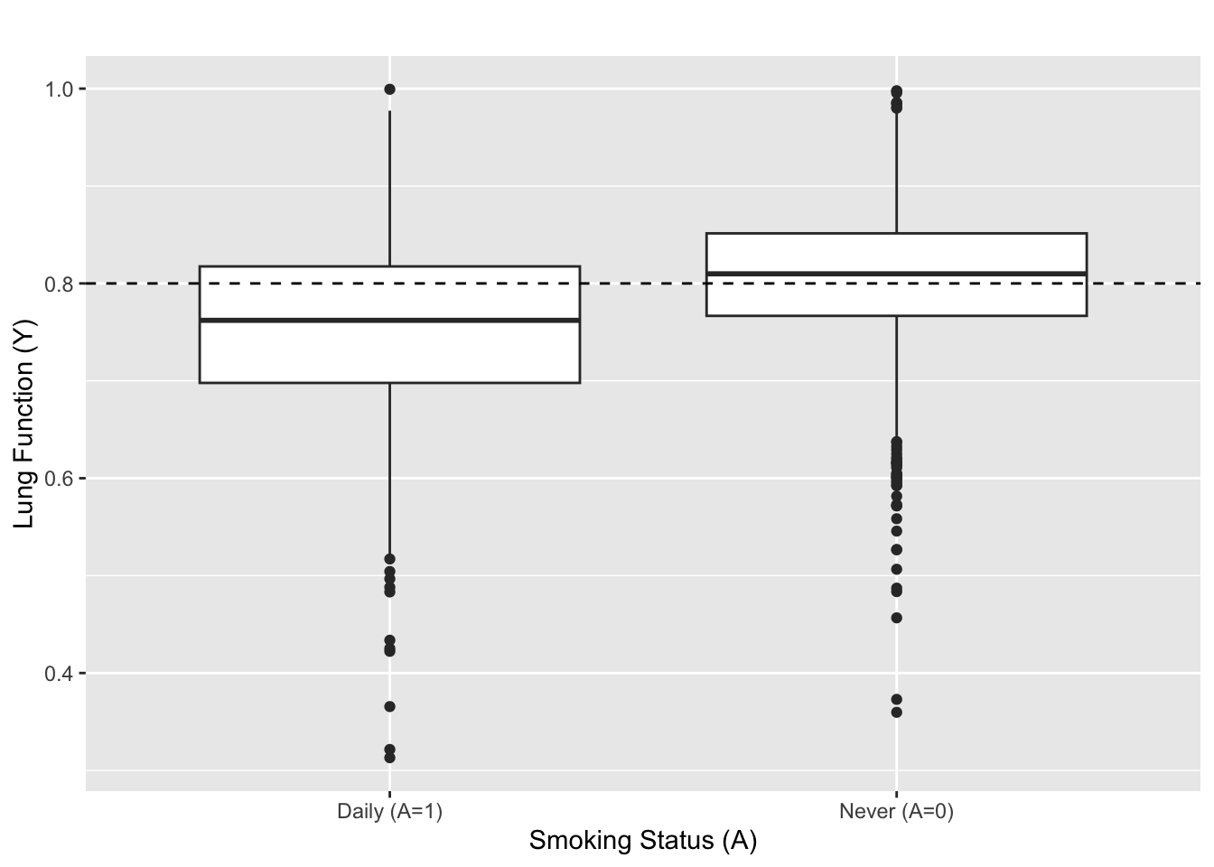
  • Outcome (\(Y\)): ratio of forced expiratory volume in one second over forced vital capacity. \(Y \geq\) 0.8 is good lung function!
  • Sample size is \(n=\) 2360.

Association of Smoking and Lung Function

library(ggplot2) 
ggplot(smoking,aes(x=smoke,y=ratio)) + geom_boxplot() + 
  labs(x="Smoking Status (A)",
       y="Lung Function (Y)",
       title="") + 
  scale_x_discrete(labels=c("Daily (A=1)","Never (A=0)")) +
  geom_hline(yintercept=0.8,linetype="dashed")

  • \(\overline{Y}_{\rm daily (A = 1) }=\) 0.75 and \(\overline{Y}_{\rm never (A = 0)}=\) 0.81.
  • \(t\)-stat \(=\) -11.8, two-sided p value: \(\ll 10^{-16}\)

Daily smoking is strongly associated with reduction in lung function.

But, is the strong association evidence for causality? After all, association does not imply causation…

Conceptually, we say \(A\) is associated with \(Y\) if \(A\) is informative about \(Y\)

  • If you smoke daily \((A = 1)\), then it’s likely that your lungs aren’t functioning well (\(Y\)).
  • Knowing your smoking status tells me something about your lung function.

Formally, let \(f(\cdot)\) denote the density (or mass function) of a random variable.

\(A\) is associated with \(Y\) if and only if \(f_{Y \mid A}(y | a) \neq f_{Y}(y)\) for some \(y,a\) with \(f(a) > 0\).

We’ll use the notation \(A \not\perp Y\) to denote association between \(Y\) and \(A\). Similarly, we’ll use \(A \perp Y\) to denote no association between \(A\) and \(Y\).

There are other measures of association beyond the difference in means between daily smokers and never smokers, i.e., \(\mathbb{E}[Y | A=1] - \mathbb{E}[Y | A=0]\). Some measures of association for scalar \(A\) and scalar \(Y\).

  • Population difference in means between treated and control groups: \(\mathbb{E}[Y | A=1] - \mathbb{E}[Y | A=0]\)
  • Population covariance: \({\rm cov}(A,Y) = \mathbb{E}[ (A - \mathbb{E}[A])(Y - \mathbb{E}[Y])]\)
    • If \(A\) is binary and \(0 < \mathbb{P}(A = 1) < 1\), \({\rm cov}(A,Y) = {\rm Var}(A) ( \mathbb{E}[Y|A=1] - \mathbb{E}[Y|A=0])\)
  • Population regression parameter: The slope parameter \(\beta_1^*\) from the population regression equation \[\begin{align*} \beta_0^*, \beta_1^* &= {\rm argmin}_{\beta_0, \beta_1 \in \mathbb{R}} \mathbb{E}[ (Y - \beta_0 - A\beta_1)^2] \end{align*}\] Some algebra reveals that \(\beta_1^* = \frac{{\rm Cov}(A,Y)}{{\rm Var}(A)}\).

Note that the population regression parameter does not assume that \(Y\) is a linear function of \(A\). Instead, \(\beta_0^*, \beta_1^*\) can be thought of as the intercept and slope of the ``best linear approximation’’ regression line between \(Y\) and \(A\). For more discussion related to this, see Section 3.1 of Buja et al. (2019) and Figure 1 of Suk and Kang (2022) for a visual illustration.

The derivation of \(\beta_1^*\) follows either from the theory of linear regression or multivariable calculus. For example, the solution to the minimize must satisfy the equation \(0 = \nabla_{\beta_0, \beta_1} \mathbb{E}[ (Y - \beta_0 - A\beta_1)^2] \bigg|_{\beta_0 = \beta_0^*, \beta_1 = \beta_1^*}\), which simplify to \[\begin{align*} 0 = \nabla_{\beta_0, \beta_1} \mathbb{E}[(Y-\beta_0)^2] + \beta_1^2 \mathbb{E}[A^2] - 2\beta_1 \mathbb{E}[(Y-\beta_0)A] \bigg|_{\beta_0 = \beta_0^*, \beta_1 = \beta_1^*} \end{align*}\] Solving for this equation leads to the familiar equation for the regression parameter: \[\begin{align*} \begin{pmatrix} \beta_0^* \\ \beta_1^* \end{pmatrix} &= \begin{pmatrix} 1 & \mathbb{E}[A] \\ \mathbb{E}[A] & \mathbb{E}[A^2] \end{pmatrix}^{-1} \begin{pmatrix} \mathbb{E}[Y] \\ \mathbb{E}[AY] \end{pmatrix} \end{align*}\]

We can estimate the population quantities by their sample counterparts (e.g., sample means, sample covariance, OLS).

Building Intuition for Causality: The Parallel Universe Analogy

Inspired by recent Marvel movies, I find the parallel universe analogy helpful to conceptualize causal effects.

Consider a particular snapshot in time (e.g., June 1, 2024, John’s 25th birthday) in two parallel universes.

  • In universe 1, John is a daily smoker.
  • In universe 2, John never smoked.
  • Beyond smoking status, everything is identical between universe 1 and 2 (John’s age, friends, parents, diet, etc.)

Now suppose John’s lung functions are different between the two universes.

  • The difference in lung functions can only be attributed to the difference in smoking status.
  • Why? All variables (except smoking status) are the same between the two parallel universes.
  • Between the two parallel universes, any difference in the outcomes must be due to a difference in the treatment status.

A helpful Youtube clip from movie Sliding Doors.

Counterfactual/Potential Outcomes

Let’s define the outcomes from the two parallel universes, often referred to as counterfactual or potential outcomes1.

  • \(Y(1)\): lung function that would have been observed if you smoked daily (i.e., parallel world where you smoked)
  • \(Y(0)\): lung function that would have been observed if you did not smoke (i.e,. parallel world where you didn’t smoke)

Similar to the observed data table, we can create counterfactual/potential outcomes data table.

\(Y(1)\) \(Y(0)\)
John 0.54 0.94
Sally 0.91 0.91
Kate 0.81 0.60
Jason 0.60 0.84

Our First Causal Effect: Individual Causal Effects

Let’s take a look at \(Y_{\rm John}(1) - Y_{\rm John}(0) = -0.4\) and \(Y_{\rm Sally}(1) - Y_{\rm Sally}(0) = 0\).

  • For John, changing smoking status causes a change in his lung function since the difference between \(Y_{\rm John}(1)\) and \(Y_{\rm John}(0)\) can only be attributed to the difference in smoking status in the parallel universes.
  • Unlike John, changing Sally’s smoking status will not cause a change her lung function.

Both numbers \(-0.4\) and \(0\) are individual causal effects as they reflect each person’s change in the outcome when their smoking status changes.

When causal effects differ from individual to individual, the causal effect is generally said to be heterogeneous. If the effects are the same for every individual, the causal effect is generally said to be homogeneous or constant.

Other Measures of Causal Effects

Suppose we add additional information about the individuals

\(Y(1)\) \(Y(0)\) Age \((X_1)\) Graduated HS? \((X_2)\)
John 0.54 0.94 23 Yes
Sally 0.91 0.91 27 No
Kate 0.81 0.60 32 No
Jason 0.60 0.84 30 Yes
  • The average2 treatment effect (ATE): \(\mathbb{E}[Y(1) - Y(0)]\)
  • The conditional average treatment effect (CATE): \(\mathbb{E}[Y(1) - Y(0) | X_2 = {\rm Yes}]\)

These are examples of causal estimands/parameters because they are functions of the counterfactual outcomes.

Similar to the observed data \((Y,A)\), you can think of the counterfactual data table as an i.i.d. from some population distribution of \(Y(1),Y(0)\).

Formally, let \(F(\cdot)\) denote the cumulative distribution function of a random variable. Then, \(Y_i(1), Y_i(0) \overset{\text{i.i.d.}}{\sim} F_{Y(1),Y(0)}\))

  • This is often referred to as the super-population framework.
  • Expectations are defined with respect to the population distribution (i.e. \(\mathbb{E}[Y(1)] = \int y dF_{Y(1)}(y)\))
  • The population distribution is fixed and the sampling generates the source of randomness (i.e. i.i.d. draws from \(F_{Y(1),Y(0)}\), perhaps \(F_{Y(1),Y(0)}\) is jointly Normal?)
  • For asymptotic analysis, \(F_{Y(1),Y(0)}\) is usually fixed (i.e. \(F_{Y(1),Y(0)}\) does not vary with sample size \(n\)). In high dimensional regimes, \(F_{Y(1),Y(0)}\) will vary with \(n\).

Or, you can think of \(n=4\) as the entire population.

  • This is often referred to as the finite population/randomization inference or design-based framework.
  • Expectations are defined with respect to the table above (i.e. \(\mathbb{E}[Y(1)] = (0.5+0.8+0.9+0.6)/4 =0.7\)). The notation \(\mathbb{E}[Y(1)]\) is a bit misleading and people do not use it to denote the average of \(Y(1)\) in the finite population setup.
  • The counterfactual data table is the population and the treatment assignment (i.e. which counterfactual universe you get to see; see below) generates the randomness and the observed sample.
  • For asymptotic analysis, both the population (i.e. the counterfactual data table) and the sample changes with \(n\). In some vague sense, asymptotic analysis under the finite sample framework is inherently high dimensional.

The latter framework is uncommon in typical statistics courses. However, it’s very popular among some circles of causal inference researchers (e.g. Rubin, Rosenbaum and their students). The appendix of Erich Leo Lehmann (2006), P. Rosenbaum (2002b), and Li and Ding (2017) provide a list of technical tools to conduct this type of inference.

There has been a long debate about which the “right” framework for inference. My understanding is that it’s now (i.e. Jan. 2025) a matter of personal taste. Also, as Paul Rosenbaum puts it:

In most cases, their disagreement is entirely without technical consequence: the same procedures are used, and the same conclusions are reached…Whatever Fisher and Neyman may have thought, in Lehmann’s text they work together. (Page 40, P. Rosenbaum (2002b)

The textbook that Paul is referring to is (now) Erich L. Lehmann and Romano (2006). Note that this quote touches on another debate in the literature in finite-sample inference, which is what is the correct null hypothesis to test. In general, it’s good to be aware of the differences between the two frameworks and as Lehmann did (see full quote), use the strengths of each different frameworks. For some interesting discussions on this topic as it relates to causal inference, see Robins (2002), P. Rosenbaum (2002a), Chapter 2.4.5 of P. Rosenbaum (2002b), and Abadie et al. (2020). For more well-known works in the area of finite population inference, see Neyman (1923), Freedman and Lane (1983), Freedman (2008), and Lin (2013).

Average Treatment Effect (i.e., the Causal Effect)

Let’s consider the ATE \(\mathbb{E}[Y(1) - Y(0)]\), by far the most popular causal estimand/measure of a causal effect.

  • This is the average of John’s, Sally’s, etc. causal effects of smoking on lung function.

If this average is zero, then on average, the causal effect of smoking on lung function is zero.

  • This doesn’t mean that everyone’s individual causal effect is zero.
  • Some people may have a positive individual causal effect, others may have a negative individual causal effect, and some may have zero individual causal effect.

If this average is negative, then being a daily smoker is, on average, cause decrease in lung function compared to being a never-smoker.

By linearity of expectations, \(\mathbb{E}[Y(1) - Y(0)] = \mathbb{E}[Y(1)] - \mathbb{E}[Y(0)]\).

  • In words, the average of everyone’s causal effects is also the difference in the average of everyone’s lung functions when they are daily smokers (i.e., \(\mathbb{E}[Y(1)]\)) versus when they are never smokers (i.e., \(\mathbb{E}[Y(0)]\)).
  • While the equality is trivial, it allows us to study the ATE by studying the marginal distributions of \(Y(1)\) and \(Y(0)\) rather than studying the joint distribution of \(Y(1), Y(0)\).

What’s the difference between \(\mathbb{E}[Y | A=1]\) versus \(\mathbb{E}[Y(1)]\)?

  • \(\mathbb{E}[Y|A=1]\) is the average of the observed lung function among those who are daily smokers (i.e., \(A=1\)).
  • \(\mathbb{E}[Y(1)]\) is the average of the counterfactual lung function had everyone been a daily smoker (i.e., the \(1\) inside \(Y(1)\)).

Some Subtle Points about Causal Effects

  1. Causal effects of a treatment is often defined as a comparison to another (possibly inactive) treatment.

    • In addition to linear differences,causal effects can also be defined as contrasts in log scale, \(\log(Y(1)) - \log(Y(0))\) so long as \(Y(0),Y(1)\) are positive.
    • See Chapter 1.3 of Hernán and Robins (2020) for details.
  2. We focus on the effects of causes (e.g., effect of daily smoking on lung function) rather than the causes of effects (e.g., why does John have poor lung function?). The causes of effects are hard to define because of the problem of infinite regress.

    Example (from Don Rubin): He got lung cancer because he smoked cigarettes. The real reason he smoked is because his parents smoked, and they smoked because they hated each other and they hated each other because…

  3. Cause-effect relationships have a natural temporal ordering where the treatment variable (i.e., smoking status) always precedes the outcome variable (i.e., lung function)

    • You can’t have an effect (i.e. outcome) before a cause (i.e. treatment variable).
    • You also can’t have causal simultaneity where the outcome and treatment variable simultaneously change each others values at the exact same time. This makes it impossible to determine whether the outcome is causing the treatment variable or vice versa.
  4. (Discussed more later) The notation currently does not make a distinction between different kinds of daily smoking on lung function (e.g., John smokes 10 packs of cigars per day versus 1 cigar per day). The notation assumes no multiple versions of treatment.

To be more precise in the smoking example, we need to further define what it means to be a daily smoker and a never-smoker. For example,

  1. Is a daily smoker a person who smokes at least 1 cigarettes per day at least once a week every year?
  2. Is a daily smoker a person who smokes at least 1 pack of cigarettes per week for at least 50 weeks of the year?
  3. Is a daily smoker a person who smokes during all time in their lives, including during pregnancy?
  4. Should we only consider smoking behavior after age 21?
  5. Should we only exclude electronic cigarettes when we consider smoking behavior?

Each variation in the definition of daily smoking can change the parallel universe 1 and subsequently, the difference between John’s lung function between the two parallel universes. For example, under definition (a), the difference between John’s lung function may be \(-0.4\). But under definition (b), the difference may be \(0\), i.e., smoking status does not change John’s lung function. The two definitions yield scientifically different causal conclusions about John’s smoking status on his lung function.

Also, it’s equally important (in my personal opinion, far more important) to precisely define the never smokers, or more generally, the control group. As mentioned in the subtle points, causal effects are usually contrasts of outcomes and in the smoking example, the control group is a never smoker. If we choose an “extreme” control group, say our control group are those who not only never smoked, but never been near someone who smoked cigarettes, the difference between the outcomes among treated and control groups may be too dramatic than in most realistic settings. In fact, as we’ll discuss later, you can study biases from unmeasured confounders/selection on unobservables/etc. by selecting a good control group (e.g., P. R. Rosenbaum (1987)).

Between the control and the treatment, the treatment is usually well-defined in most policy evaluations (e.g., implementation/enactment of policy) and randomized experiments (e.g., giving a particular drug).

Finally, while not apparent right now, the definition of treatment/intervention/exposure must also be consistent across all study units; see later lecture notes. In general, causal inference requires, to some extent, a well-defined intervention/treatment/exposure to yield useful, practically meaningful causal conclusions; see fine point 1.2 in Hernán and Robins (2020). Otherwise, if there are variations in the definition of the treatment across individuals, say John’s definition of daily smoking differs from Sally’s definition of daily smoking, and we conduct a causal analysis that includes John and Sally, it would be difficult to make useful, practically meaningful causal claims about the causal effect of daily smoking.

In short, when interpreting causal effects, it is important to be cognizant of how the treatment/intervention is defined to yield unambiguous conclusions about causality.

A healthy majority of people in causal inference argue that the counterfactual outcome of race and gender are ill-defined. For example, suppose we are interested in whether being a female causes lower income. We could define the counterfactual outcomes as

  • \(Y(1)\): Jamie’s income when Jamie is female
  • \(Y(0)\): Jamie’s income when Jamie is not female

Similarly, we are interested in whether being a black person causes lower income, we could define the counterfactual outcomes as

  • \(Y(1)\): Jamie’s income when Jamie is black
  • \(Y(0)\): Jamie’s income when Jamie is not black

But, if Jamie is a female, can there be a parallel universe where Jamie is a male? That is, is there a universe where everything else is the same (i.e. Jamie’s whole life experience up to 2025, education, environment, maybe Jamie gave birth to kids), but Jamie is now a male instead of a female? This question is related to the question of manipulability of treatment.

In the intuitive understanding of experimentation that most people have, it makes sense to say, “Let’s see what happens if we require welfare recipients to work”; but it makes no sense to say “Let’s see what happens if I change this adult male into a three-year-old girl.” And so it is also in scientific experiments. Experiments explore the effects of things that can be manipulated, such as the dose of a medicine, the amount of a welfare check, the kind or amount of psychotherapy or the number of children in a classroom. Nonmanipulable events (e.g., the explosion of a supernova) or attributes (e.g., people’s ages, their raw genetic material, or their biological sex) cannot be causes in experiments because we cannot deliberately vary them to see what then happens. Consequently, most scientists and philosophers agree that it is much harder to discover the effects of nonmanipulable cause. (Page 8 of Shadish, Cook, and Campbell (2002)).

Note that we can still measure the association of gender on income, for instance with a linear regression of income (i.e \(Y\)) on gender (i.e. \(A\)). This is a well-defined quantity.

There is an interesting set of papers on this topic: VanderWeele and Robinson (2014), Vandenbroucke, Broadbent, and Pearce (2016), Krieger and Davey Smith (2016), VanderWeele (2016). See Volume 45, Issue 6, 2016 issue of the International Journal of Epidemiology. Some even take this example further and argue whether counterfactual outcomes are well-defined in the first place; see Dawid (2000) and a counterpoint in Sections 1.1, 2 and 3 of Robins and Greenland (2000).

Counterfactual Data Versus Observed Data

Table 1: Comparison of tables.
(a) Counterfactual table
\(Y(1)\) \(Y(0)\)
John 0.54 0.94
Sally 0.91 0.91
Kate 0.81 0.60
Jason 0.60 0.84
(b) Observed table
\(Y\) \(A\)
John 0.94 0
Sally 0.91 0
Kate 0.81 1
Jason 0.84 0

In the counterfactual table, we see what everyone’s lung function would be if they are never-smokers and daily smokers.

  • Comparing John’s \(Y(1)\) and \(Y(0)\) gives us John’s causal effect of being a daily smoker versus a never-smoker on his lung function.
  • Similary, comparing Sally’s \(Y(1)\) and \(Y(0\)) gives us Sally’s causal effect of being a daily smoker versus a never-smoker on her lung function.

In the observed table, we only see everyone’s lung function under one particular status of smoking status.

  • We only see John’s lung function when he is a non-smoker (i.e., \(Y_{\rm John} = 0.94\) when \(A_{\rm John} = 0\)). We don’t get to see his lung function in the parallel universe when, contrary to fact, he is a daily smoker.
  • Similarly, we only see Sally’s lung function when she is a non-smoker (i.e., \(Y_{\rm Sally} = 0.91\) when \(A_{\rm Sally} = 0\)). We don’t get to see her lung function in the parallel universe, when contrary to fact, she is a daily smoker.

Fundamental Problem of Causal Inference (Holland 1986)

Without additional information, it’s impossible to study causal effects from the observed data table because we don’t get to observe all counterfactual outcomes. This is the fundamental problem of casual inference (Holland 1986).

A key goal in causal inference is to learn about both counterfactual outcomes \(Y(1), Y(0)\) when you only observe one of them.

  • This often involves making (usually untestable) assumptions about the counterfactual data and/or the observed data.
  • These assumptions are often referred to as assumptions for causal identification.

The fundamental problem is closely related to a missing data problem; we’ll explore this later.

When Can You Observe Both Counterfactuals? Unit Homogeneity Assumption

There are situations in the real world where you can observe all counterfactual outcomes. Most of them take place in lab experiments or in manufacturing and all of them fundamentally rely on some domain knowledge to claim that all counterfactual outcomes are observable.

Suppose we want to determine the causal effect of putting a chocolate bar over a candle.

  • \(Y(1)\): the counterfactual outcome of the chocolate bar if it’s over a candle.
  • \(Y(0)\): the counterfactual outcome of the chocolate bar if it’s not over a candle.
  • Let’s say these outcomes measure whether the chocolate melted (1) or not (0).

We put one chocolate bar over a candle and another bar away from the candle, resulting in the following table.

\(Y(1)\) \(Y(0)\)
1st chocolate bar 1 NA
2nd chocolate bar NA 0

Despite the missing values in the potential outcomes, we can impute them from our daily experiences.

  • We know that chocolates bars are identical with respect to their behavior under heat.
  • Therefore, we can obtain the second chocolate bar’s missing \(Y(1)\) from the first chocolate bar’s \(Y(1)\).
  • Similarly, we know that chocolates don’t melt without heat and thus, we can impute the missing first chocolate bar’s \(Y(0)\) with the second chocolate bar’s \(Y(0)\).

This phenomena is known as the unit homogeneity assumption and is formalized as follows

\[Y_{i}(1) = Y_j(1) \text{ and } Y_i(0) = Y_j(0) \quad{} \forall i\neq j \] Note that we don’t even have to randomize which chocolate bar is exposed to heat or not to identify the causal effect of heat on the chocolate bar. We also don’t have to sample \(10\) or \(100\) chocolate bars to understand the causal effect of exposing chocolate to heat on melting as all chocolate bar.

References

Abadie, Alberto, Susan Athey, Guido W Imbens, and Jeffrey M Wooldridge. 2020. “Sampling-Based Versus Design-Based Uncertainty in Regression Analysis.” Econometrica 88 (1): 265–96.
Buja, Andreas, Lawrence Brown, Richard Berk, Edward George, Emil Pitkin, Mikhail Traskin, Kai Zhang, and Linda Zhao. 2019. “Models as Approximations i.” Statistical Science 34 (4): 523–44.
Dawid, A Philip. 2000. “Causal Inference Without Counterfactuals.” Journal of the American Statistical Association 95 (450): 407–24.
Freedman, David. 2008. “On Regression Adjustments to Experimental Data.” Advances in Applied Mathematics 40 (2): 180–93.
Freedman, David, and David Lane. 1983. “A Nonstochastic Interpretation of Reported Significance Levels.” Journal of Business & Economic Statistics 1 (4): 292–98.
Hernán, Miguel, and James Robins. 2020. Causal Inference: What If. Boca Raton: Chapman & Hall/CRC.
Holland, Paul. 1986. “Statistics and Causal Inference.” Journal of the American Statistical Association 81 (396): 945–60.
Krieger, Nancy, and George Davey Smith. 2016. “The Tale Wagged by the DAG: Broadening the Scope of Causal Inference and Explanation for Epidemiology.” International Journal of Epidemiology 45 (6): 1787–1808.
Lehmann, Erich Leo. 2006. Nonparametrics: Statistical Methods Based on Ranks. Springer.
Lehmann, Erich L, and Joseph P Romano. 2006. Testing Statistical Hypotheses. Springer.
Li, Xinran, and Peng Ding. 2017. “General Forms of Finite Population Central Limit Theorems with Applications to Causal Inference.” Journal of the American Statistical Association 112 (520): 1759–69.
Lin, Winston. 2013. Agnostic notes on regression adjustments to experimental data: Reexamining Freedman’s critique.” The Annals of Applied Statistics 7 (1): 295–318.
Neyman, Jerzy. 1923. “On the Application of Probability Theory to Agricultural Experiments. Essay on Principles. Section 9.” Statist. Sci. 5 (4): 465–72.
Robins, James M. 2002. “Covariance Adjustment in Randomized Experiments and Observational Studies: Comment.” Statistical Science 17 (3): 309–21.
Robins, James M, and Sander Greenland. 2000. “Causal Inference Without Counterfactuals: Comment.” Journal of the American Statistical Association 95 (450): 431–35.
Rosenbaum, Paul. 2002a. “Covariance Adjustment in Randomized Experiments and Observational Studies.” Statistical Science 17 (3): 286–327.
———. 2002b. Observational Studies. Springer.
Rosenbaum, Paul R. 1987. “The Role of a Second Control Group in an Observational Study.” Statistical Science 2 (3): 292–306.
Rubin, Donald B. 1974. “Estimating Causal Effects of Treatments in Randomized and Nonrandomized Studies.” Journal of Educational Psychology 66 (5): 688.
Shadish, W. R., T. D. Cook, and D. T. Campbell. 2002. Experimental and Quasi-Experimental Designs for Generalized Causal Inference. Houghton, Mifflin, & Company.
Suk, Youmi, and Hyunseung Kang. 2022. “Robust Machine Learning for Treatment Effects in Multilevel Observational Studies Under Cluster-Level Unmeasured Confounding.” Psychometrika 87 (1): 310–43.
Vandenbroucke, Jan P, Alex Broadbent, and Neil Pearce. 2016. “Causality and Causal Inference in Epidemiology: The Need for a Pluralistic Approach.” International Journal of Epidemiology 45 (6): 1776–86.
VanderWeele, Tyler J. 2016. “Commentary: On Causes, Causal Inference, and Potential Outcomes.” International Journal of Epidemiology 45 (6): 1809–16.
VanderWeele, Tyler J, and Whitney R Robinson. 2014. “On the Causal Interpretation of Race in Regressions Adjusting for Confounding and Mediating Variables.” Epidemiology 25 (4): 473–84.
Footnotes

  1. The framework was developed by Neyman (1923), republished in Statistical Science in 1990, and Rubin (1974). See Holland (1986) for more background.↩︎

  2. Expectations are defined with respect to a joint cumulative distribution function \(F_{Y(1),Y(0)}\) (i.e., super-population framework).↩︎