Justin Tritz Final Project

Feature Detection & Tracking

In many of the algorithms we talked about in class, there was some form of detecting key points in one image and trying to find the corresponding point in another image. In HW3 we were given the KLT Tracker and were told to use it as a black box for detecting and tracking features. For this project, I will figure out how to accomplish feature detection and feature tracking with my own algorithm. Once the features are detected and tracked from one image to the next, I will use those tracked features to mosaic the images. The nice thing about the algorithm I developed is it doesn’t require the images to be overlapping by a lot. I have an example of two images that are overlapping by about 50% and the algorithm was able to create a good mosaic. The algorithm is scale invariant, rotational invariant, and intensity invariant.

I will start with the feature detection algorithm which is based heavily on the intuition of what I think I would do if I was searching an image for key points. A point is a single circular region that is distinct from its surrounding region. Therefore that is the first thing I would look for. The next best key point would be like an endpoint and corners would follow endpoints (the sharper the corner the better). We can skip the idea of finding end points and treat them as very sharp corners. So what do these things have in common? A single point with a relatively constant surrounding region will have all of its gradients either pointing in or out (positive or negative gradients). Corners will not have the same gradient direction all around, but they will have the same gradient direction over some angle from 180-360 degrees depending on the sharpness of the corner.

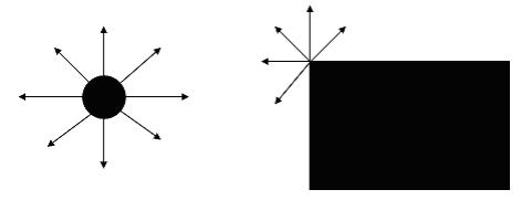
My algorithm is based entirely on these observations. For each point in the image, it computes the gradient in D directions. A point is better than another point if it has a longer chain of gradients with the same sign (positive or negative). In order to limit noise, the gradient must be of a certain magnitude to continue the chain. For example, if I have 3 gradients that are negative next to a gradient that is negative, but not of significant magnitude, then the chain length is 3. I found that requiring the magnitude to be at least 1/8 of the difference between the largest and smallest pixel values in the image works well. So if the darkest pixel is 30 and the lightest pixel is 230, the magnitude threshold would be 200/8 = 25. To actually compute the gradients, you must have a value for the center pixel and a value for some points on the border of a circle centered on the pixel. I computed each of these values based on a region centered on the pixel. The following image illustrates how gradients are computed.

We are computing the gradients for the pixel in the very center. The value for the pixel in the very center is the value of the area inside the smaller circle surrounding the center pixel. The value of that circle is a weighted sum of the pixels inside the circle, and the weights are determined by the distance the pixel is from the center pixel. The values of the points on the larger circle are calculated the same way as the value of the center circle, but we must use bilinear interpolation because those values may not be exactly centered on a pixel (they are real values). Once you know the value of the center pixel, and the values of equally spaced points on the larger circle, you can calculate the gradient in that direction by taking the difference of the two. The radius of the smaller circles are always ½ the radius of the larger circle. I chose to do this because it worked well. Also, to save on computation time, I pre-computed the values of each pixel and then used bilinear interpolation on the values calculated during the pre-computation to determine the region values during the computation. In order to get scale invariance, I would pass over the image with varying sizes of the larger circle. This works because if one image I1 is twice as big as another image I2, then you will find the same point with a circle twice as large as the circle being used when you found the point in I2. It is rotationally invariant because we are looking for the longest chain, and the rotation of a point in the image will not affect this measure. The more directions you compute the gradient in, the better. For all examples in this project, I computed the gradient in 64 directions. It is intensity invariant because the gradient is based in the difference between the center value and its surrounding values, and if they all change by the same amount, then the gradient is not affected. The gradient threshold would also be unaffected by the intensity change. A final small detail that I would like to mention is I found the algorithm to work better when I was working with a difference of Gaussian for an image, rather than the raw image pixel values. Below are some results of this feature detection algorithm on various images.

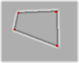
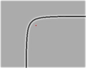
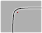
These are the key points detected for a simple square and that same square warped. As you can see, the 4 corners are detected in both cases. This is a key point detected on a curve, and that same curve scaled to ½ the size. Both points were detected with the same parameters. There were multiple passes on the image with increasing circle radius. The first point was detected with a circle of radius 32 and the second with a circle of radius 16.

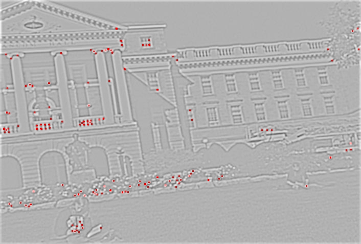
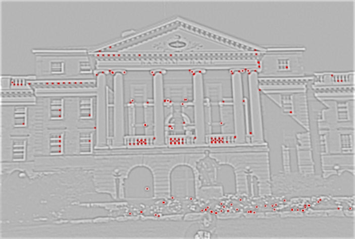
The images you see on the previous page are points detected on two images that are overlapping, but not overlapping by as much as was required for what we did in HW3. As you can visually verify, there are several points found in both images that correspond to each other.

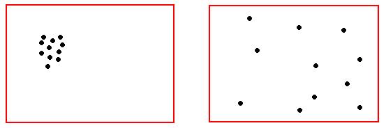
I will now go on to the feature tracking algorithm, and show that these two images can be meshed by tracking features from the first image to the second. Once again I relied on intuition to come up with an algorithm for tracking points from one image to the next. When I look at the two images above and attempt to figure out which points correspond to which points, I look for two points A and B that are surround by other points in a similar pattern. My algorithm compares all the points in the first image to all the points in the second image, and finds matches based on the geometric relationship between the point and other key points close by. If two points have a similar geometric relationship to surrounding points within their respective images, then there is a match. The way I chose to do this is choose the N closest points to the points being compared, and for the most part I found it very helpful to have N be kind of large. This makes it more difficult to find a spurious match. Obviously the best matches are the ones reported. In order to determine and compare geometric relationships, you need a method that will normalize the geometry. It must normalize the geometry based on rotation and scale in order to be consistent with what I stated earlier about this approach being rotational and scale invariant. To accomplish the rotational invariance, I calculate a major direction and rotate all points according to that major direction. If I do this for both images, then the method is rotationally invariant. I determine the major direction simply by identifying the largest gradient. This should be the same for two points that are supposed to be the same point. Once the points are rotated, the distance must be normalized in order to have scale invariance. I normalized the distance by dividing by the average distance for the N points closest to the point. I didn’t use max-min in order to avoid outliers causing problems. Once the N closest points are detected, rotated, and scaled, if the two points correspond to each other, the points should come very close to overlaying each other. To compute how well the points overlay each other, I compute the distance from every point in the first image to the point closest to it in the second image, and do the same for the second image to the first image. The reason I do this in both directions is to avoid a small distance when 1 point in 1 image is close to all the points in another image, but the rest of the points are far away. Below is an example of what I am trying to avoid.

If I only determined distance as the distance from all points in the first image to the closest point in the second image, these images would be considered close to overlaying each other. Obviously that would be bad.

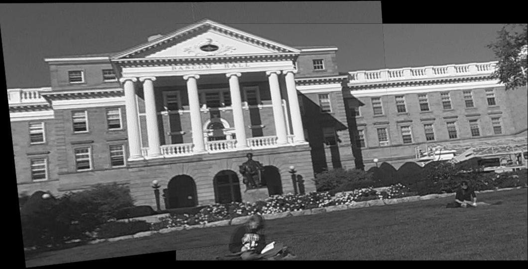
As you can see, these two images are not overlapping by as much as you might think they would need to. The features used as input to the feature tracking algorithm were the features you can see in the earlier images in this paper.

This is a mosaic that did not work for me on HW3, but worked when I used the algorithms in this paper.

As you can see, the algorithms do work. I am sure they can be improved on since they have only been in existence in my mind for a short amount of time. It is entirely possible that others have explored this idea as well, but I have not seen anything like it. Overall, this was a very enjoyable project. I like developing my own thoughts much more than trying to understand what others were thinking when they created something, and that is what I was able to do here.

Source Code