Feature Extraction

To extract the observed states, transitions, and examples from the automaton image, we use “classical” computer vision techniques, relying heavily on morphological properties to distinguish the relevant features of the image. In particular, we detect states and example boxes through their circularity (resp. rectangularity), and arrows through their endpoints and orientation.

Medium Challenges

Engineering these features proved to be a challenging problem, mostly related to the medium: whiteboards are often dirty in practice, creating an uneven “whiteboard noise”, compounded by messy drawing and uneven marker strokes. This leads to signifiant reliance of heuristics to clean and distinguish features. However, we were ultimately able to engineer features which worked consistently across all our example images.

Whiteboard Noise

Examining the background of any of the sample automata featured on this site illustrates the challenge of “whiteboard noise”. The backgrounds are often unevenly lit, featuring partially erased marks from previous drawings, as well as “ghost” lines, where a previously-marked line was erased more fully than the surrounding background.

Figure 1: Full color, grayscale, thresholded, and cleaned whiteboard images, shown here for transition detect, with states and examples masked out.

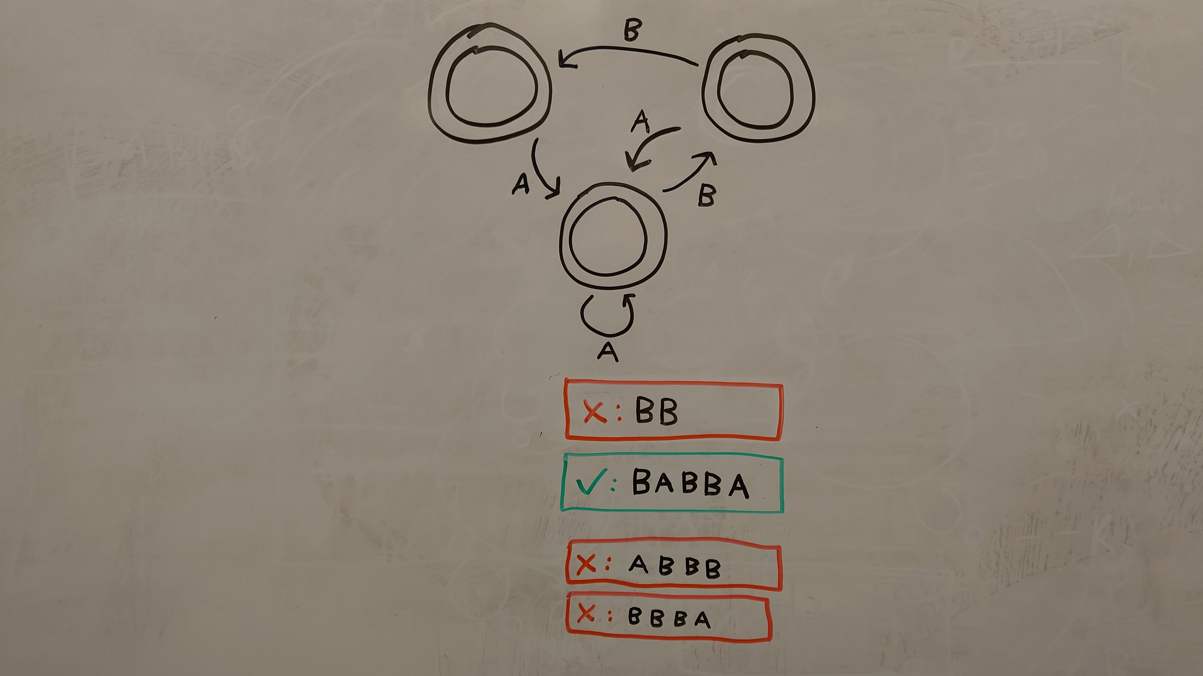
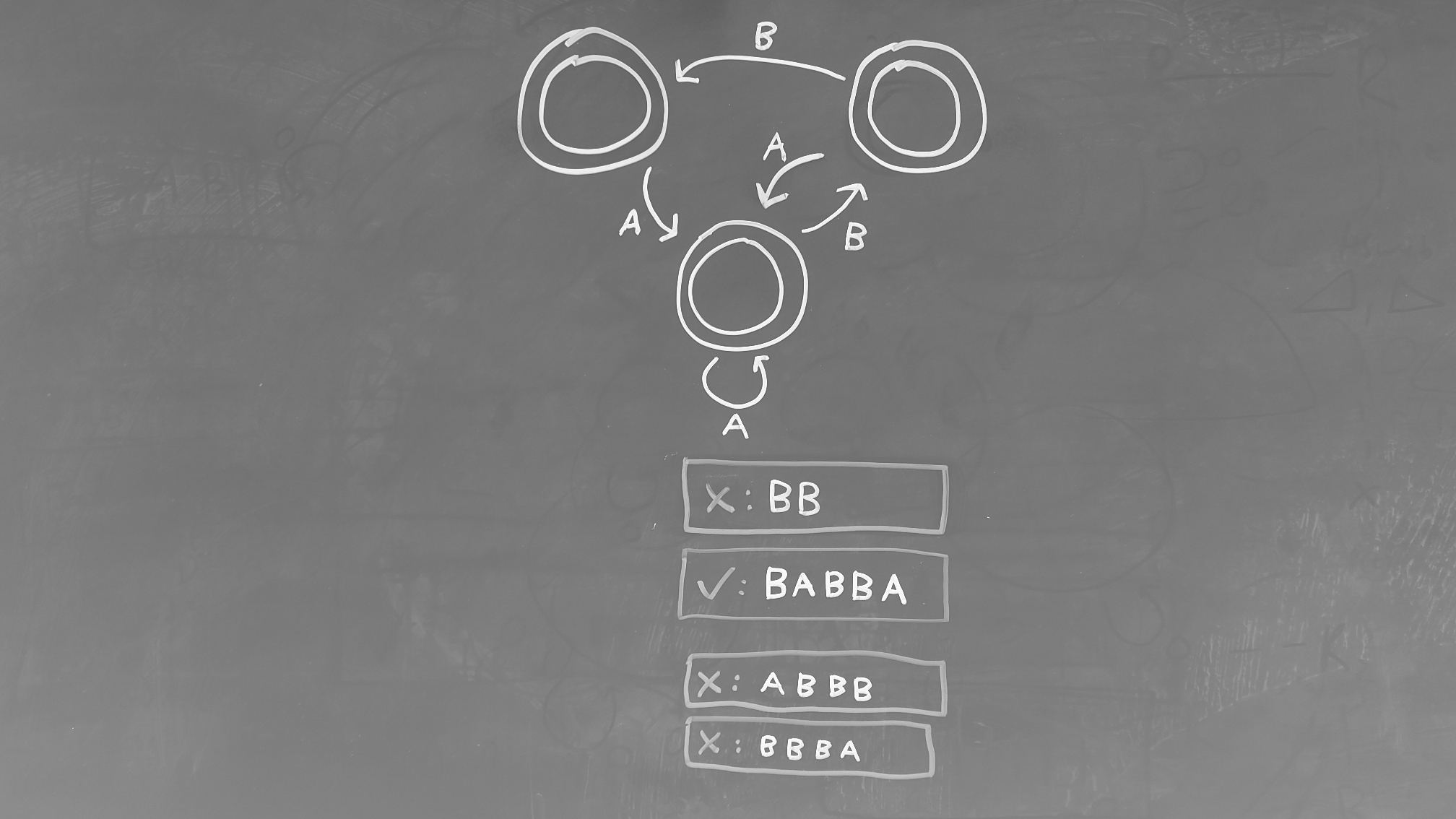
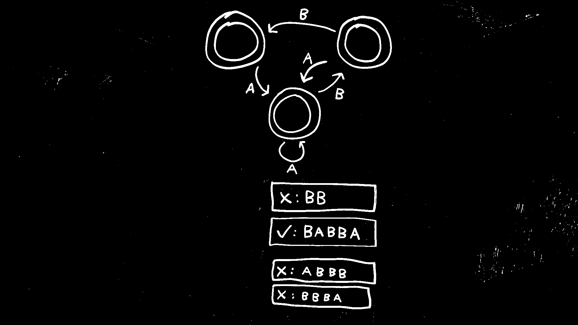
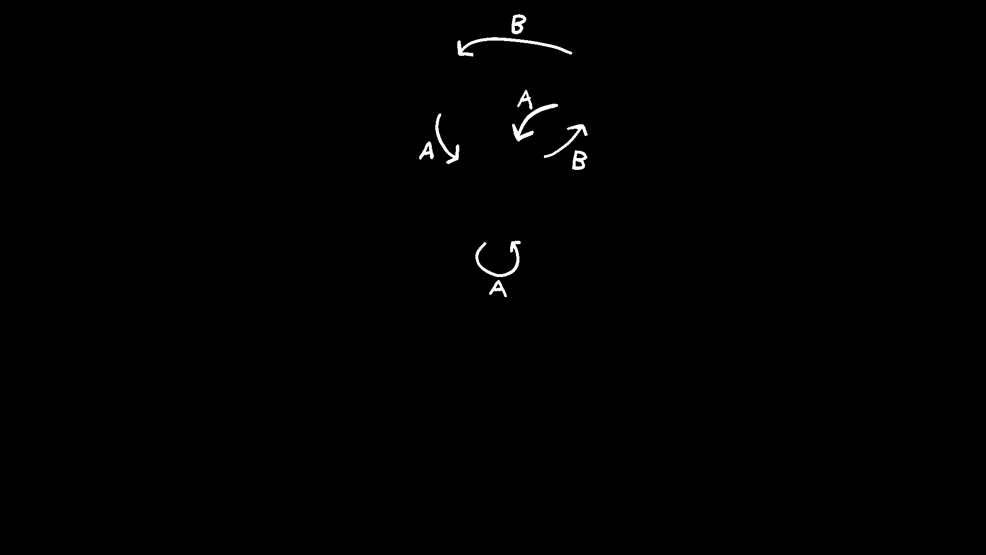
Figure 1 shows images of an automaton through the cleaning process. After inverting and converting to grayscale, the image is binarized using an adaptive threshold. While this eliminates much of the whiteboard noise, there are notable areas remaining. These are tackled by iteratively applying a Gaussian blur to the image and thresolding to create a mask, applied to the binarized image. For features later in the pipeline, already recognized features are also masked out (e.g., states and examples when detecting transitions).

Squiggly Lines

Another challenge presented by whiteboards is that the diagrams are hand-drawn, meaning circles are only roughly circular and lines are only approximately straight (Figure 2). Additionally, the marker strokes are uneven and include missing streaks. Together, this makes using standard techniques like Hough transforms and corner detectors difficult at best. Much of the challenge comes from finding methods that can robustly identify the various diagram pieces despite their imperfections.

Figure 2: Circles are approximately circular and lines are approximately straight, which proves to be a challenge.

Feature Engineering

The following sections summarize how the three primary features were detected. Our features are predicated on the assumption that any feature of interest is completely connected to itself and disconnected from other features. This means that each connected regions can be processed in isolation (other than labels associated with transitions).

States

The most reliable way of detecting state circles was by filling each region and computing its circularity. Despite their often egg-shaped-ness, state circles consistently have a circularity over 0.9. To eliminate false positives like zeros, only regions with a radius larger than half of the largest region are marked as states.

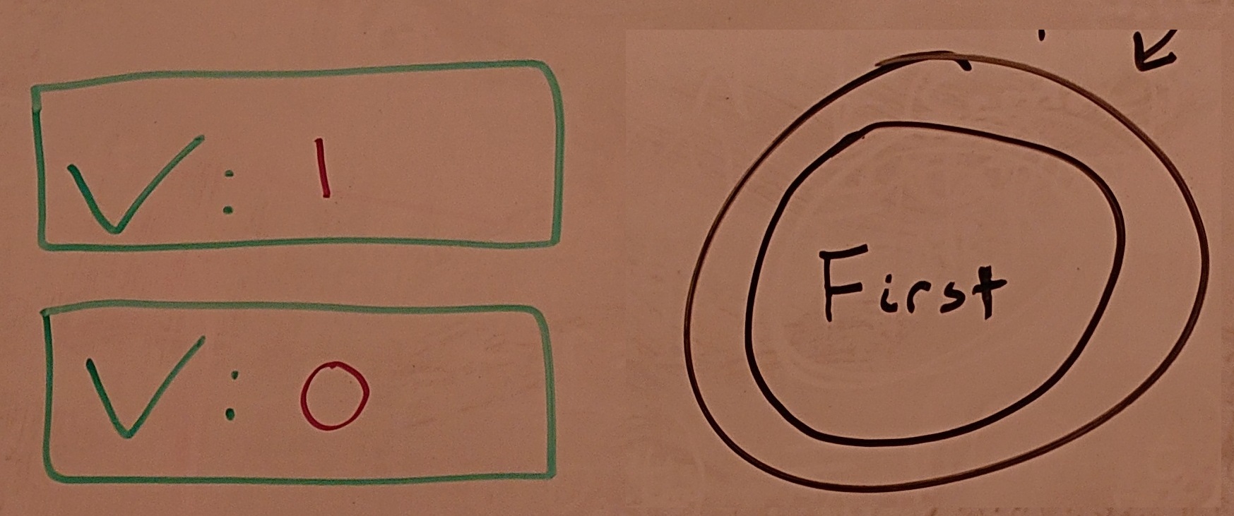
To detect accepting states (two concentric circles), we compute the intersecting area of all states. Any state that completely encloses another state is marked as an accepting state, and the inner state ignored. Note that any text inside of states (as seen on many of the example automata) is ignored.

Examples

All input examples are enclosed in a box, colored red for negative examples and green for positive examples. We filter the image by color to get the boxes, and perform a similar process to state detection, except filtering on rectangularity for example boxes.

After detecting the boxes, we OCR every region inside of the box to build up the example string. The initial “X” or checkmark is discarded, and the remaining regions are treated as characters. Due to flakiness of the OCR process (as trained on images of 0, 1, A, and B written on the whiteboard), the OCR process includes considerable heuristics to correct for the observed inaccuracy.

For example, the trained OCR model has a difficult time distinguishing between B and 1. If the model reports a character as a B with low confidence, we compute the aspect ratio of the region. If it is tall and skinny, then the character is flipped to a 1. Despite the apparent fragility of these heuristics, they significantly improved the consistency of the OCR process.

Transitions

To detect arrows, we perform a series of various morphological operations to skeletonize the region, while handling various observed sources of noise. For example, some arrows end up with slits due to the inconsistency of whiteboard marker strokes. We combat this by performing morphological closing with disks of increasing radius until the region contains no holes (or a limit is reached).

After skeletonization, we look for the three endpoints: one at the base of the arrow, and two forming the head, which are in close proximity (via region pixels). From these endpoints, we compute mid- and quarter-points. These are projected backward and forward to find the closest intersecting states.

Figure 3: Arrows with endpoints, midpoint, and quarterpoints shown. The cyan line is projected backwards to find the originating state, and the magenta line is projected forward to find the resulting state.

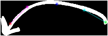
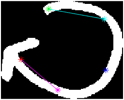
Figure 3 shows two arrows with these points and lines annotated. The cyan line is projected back until reaching a state to find the state that the transition is coming from, and the magenta line is projected forward to find the state being transitioned to.

Finally, the transition label is found by finding the closest region to the center of the transition. This region (if above a certain size threshold) is processed through OCR and returned as the transition label.