Brandon M. Smith

Outline

Introduction
Approach
Results
List of Submitted Files
References

Introduction

Several algorithms were used and implemented for this project, including those for:

A. Removing radial distortion
B. Warping images onto cylindrical coordinates
C. Finding Scale Invariant Feature Transform (SIFT) points
D. Matching these points between adjacent images
E. Random Sample Consensus (RANSAC) for finding suitable homographies
F. Image transformation
G. Image Stitching

Approach

All of the “code” used for this project was written in MATLAB. This was convenient since MATLAB – the Image Processing Toolbox in particular – has many built-in functions that make some tasks easier. A good example of this is image transformation. MATLAB conveniently provides an imtransform function that nicely transforms images, with nice sampling and reconstruction (i.e., using bicubic interpolation, which is what I used).

The main MATLAB script is mosaic.m and is located in the “program” directory. It is used like this:

result_img = mosaic(filename, f, k1, k2);

where

result_img is the panoramic mosaic result
filename is the name of a text file that contains a list of all of the image files that will go into the panorama.
f is the focal length. In our case, since we used the Canon A640 with tag 4726208885 at 480x640 resolution, f = 663.3665.
k1 and k2 are radial distortion coefficients. In our case they were k1 = -0.19447 and k2 = 0.23382

Three portions of this assignment were not written by me. I did not write the script for correcting radial distortion (see rect.m), getting an initial set of matching points between images (match.m), or the script for finding SIFT features (sift.m).

For image stitching, I used a technique suggested by the TA, Yu-Chi. The amount of contribution by each original pixel to the final pixel at each location is determined by a weighted average. The weights are calculated based on the squared distance from each pixel to its corresponding image center. So, given img1 and img2, the resulting pixel would be

( 1/r1^2 * p1 + 1/r2^2 * p2 ) / (1/r1^2 + 1/r1^2)

where r1 and r2 are the distances from the center of img1 and img2 to p1 and p2 respectively, and p1 and p2 are pixel values from img1 and img2 respectively.

Results

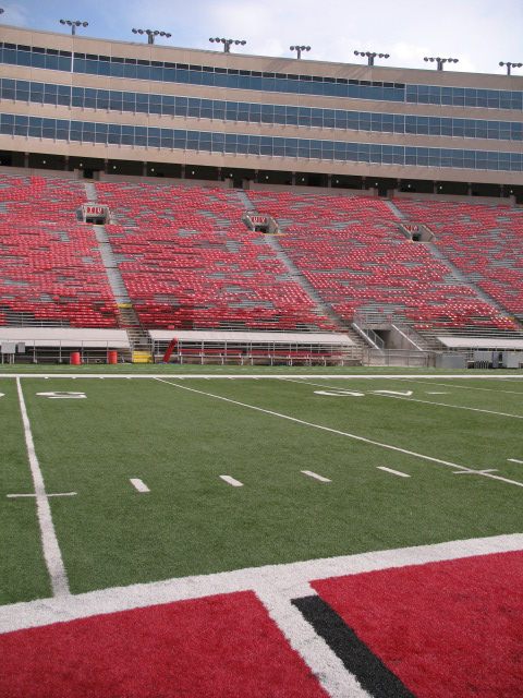
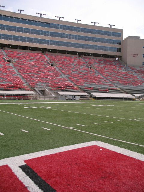
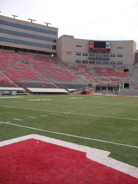
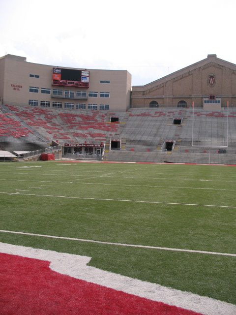
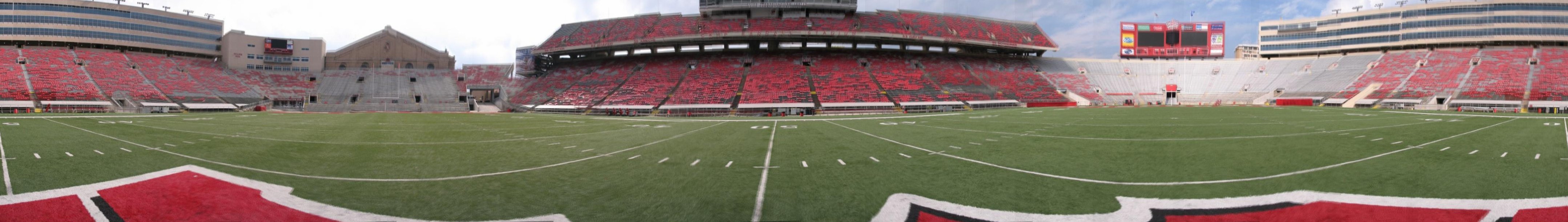
Chris Hinrichs and I took pictures at several locations in and around campus, including the center of Camp Randall Stadium, the hill in Camp Randall, a hallway in Engineering Hall, the Union (not shown), the fountain outside Memorial Library, and State Street (not shown). These images are shown in Figures 1 – 3, and 5. My favorite image is shown in Figure 1.

Figure 1: Camp Randall Stadium
a. individual images

b. panoramic mosaic image (favorite image)

c. applet

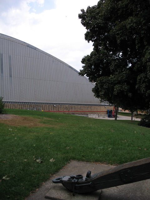
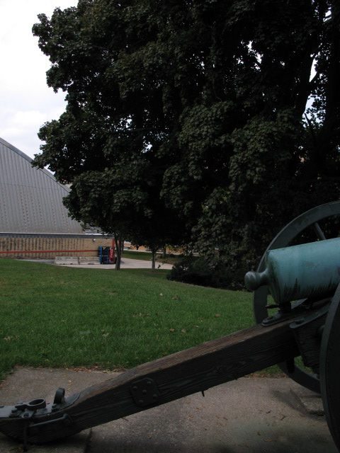
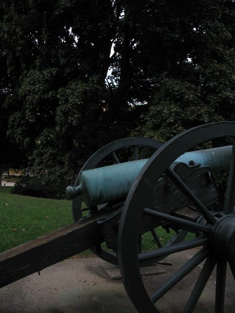
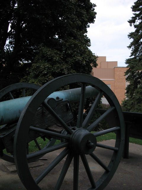
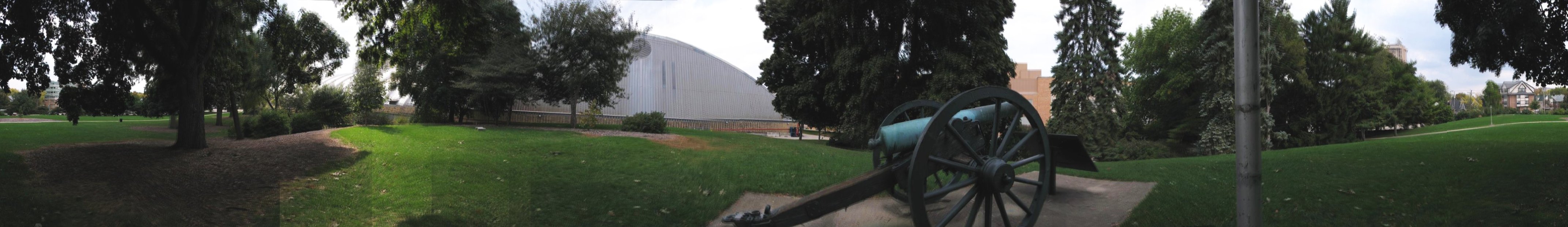
Figure 2: the hill in Camp Randall
a. individual images

b. panoramic mosaic image

c. applet

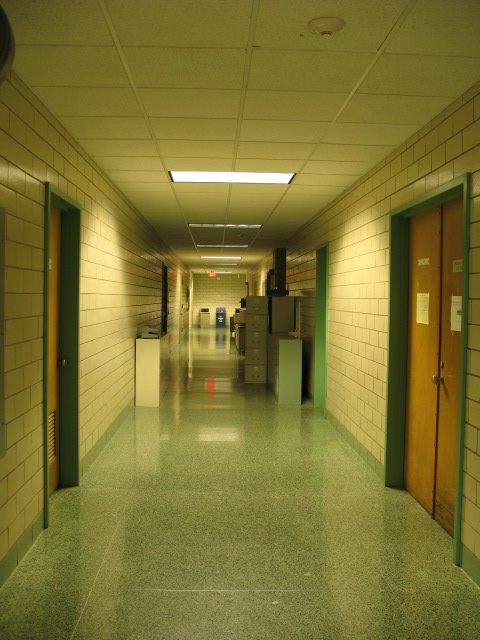
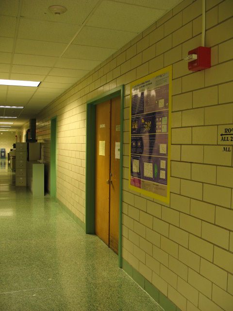
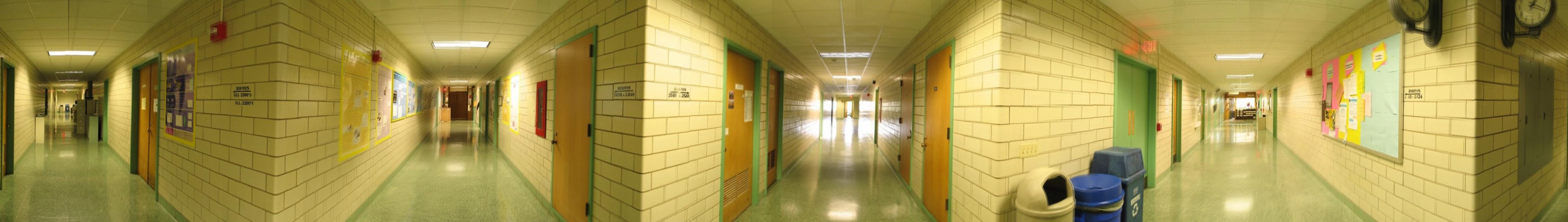
Figure 3: inside Engineering Hall
a. individual images

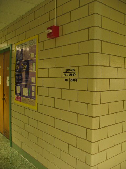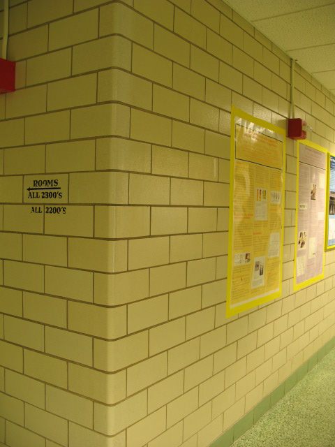b. panoramic mosaic image

c. applet

The test image was used first to create a panorama. The result is shown in Figure 4. Notice the gradual slant down and to the right. The previous images had the same problem, but this was corrected and the images cropped using the GIMP image processing software.

Figure 4: uncropped test image panorama

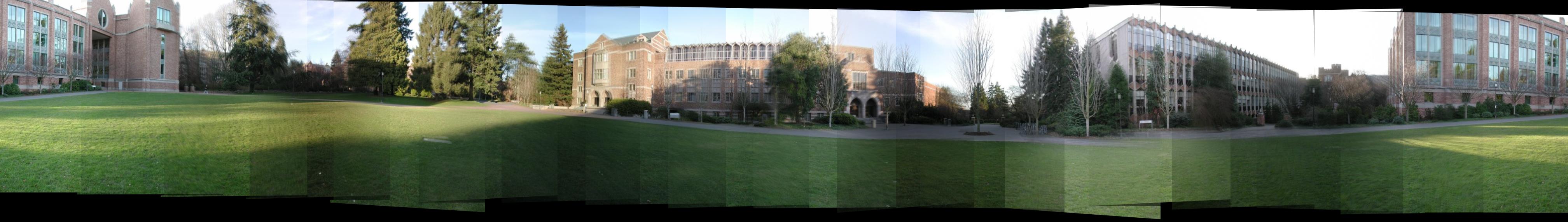
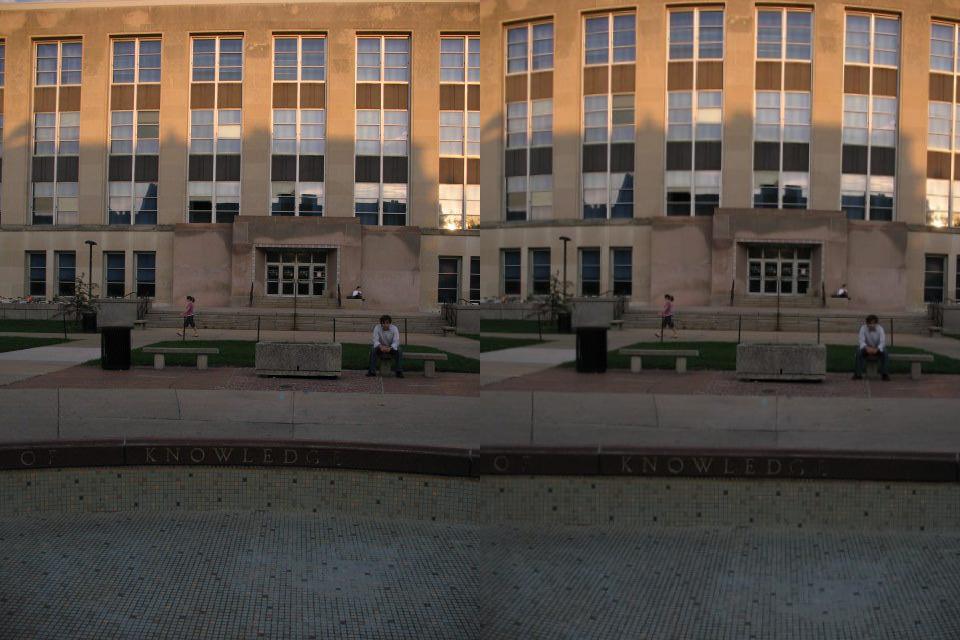
Figure 5 shows an image taken outside of Memorial Library from the center of the found. It illustrates the effect of warping. Notice in the original image on the left the fountain ledge, which is obviously curved. However, if a panorama is to be made, this ledge should span the entire 360 degree image in a straight line. The warped image on the right shows this clearly.

Figure 5: example of warping - unwarped (left) and warped (right)

The results obtained were reasonably good. However, some blurring is visible, especially near the top and bottom of the panorama. This may be due, in part, to slight imperfections in the camera calibration, i.e., f and k1 and k1 might not be totally accurate. It may also be caused by non-ideal transformations, i.e., the homography chosen by the algorithm might not be the most ideal one. The images were generated with k = 50 and the threshold set to 2 pixels. Better results could probably be obtained by calculating an average of the best homographies discovered, or perhaps by setting k higher (the number of attempts at finding a homography), or by altering the threshold.

List of Submitted Files

images/ (directory)

hallway/ (directory)

Contains a set of images taken in a hallway inside Engineering Hall.

hill/ (directory)

Contains a set of images taken on a hill in Camp Randall.

results/ (directory)

Contains the panoramic mosaic image results.

hallway.jpg

Panorama of inside Engineering Hall.

hill.jpg

Panorama of the hill in Camp Randall

stadium.jpg

This is my favorite result. It is a panorama of the inside of Camp Randall Stadium.

test_image.jpg

Panorama generated from the test images.

small2/ (directory)

Contains all of the test images.

stadium/ (directory)

Contains a set of images taken inside Camp Randall Stadium.

warp_example.jpg

See Figure 5 above.

program/ (directory)

appendimages.m
defs.h
LICENSE
Makefile
match.c
match.m
showkeys.m
sift*
sift.m
siftWin32.exe
util.c
tmp.key
tmp.pgm

Used by the SIFT program

apply_distortion.m
rect.m

Two files taken from [4]. They are used to correct radial distortion.

mosaic.m

The main program. See above for usage.

calc_final_homography.m

Implements RANSAC to find the homography that will “best” transform an image.

composite_images.m

Puts two images together, with dissolved edges.

get_transformed_xy.m

Simple function that returns a transformed version of x, y based on input x, y and a homography.

pad_image.m

Returns a padded version of an image, enlarged in the x- and y-directions by a specified amount.

readimages.m

Reads in all of the images listed in a text file.

solve_for_homography.m

Given a set of four matched points between two images, calculates the homography between them.

warpimg.m

Uses rect.m to correct radial distortion, then warps the image based on the focal length.

hallway_images.txt
hill_images.txt
stadium_images.txt
test_images.txt

Contain a list of image file names to be used to create a panoramic mosaic. These files can be read in by mosaic.m

README.txt

Describes very briefly how to run the mosaic program.

report.html
report.pdf
report.doc

You’re reading one of these.

References

[1] Szeliski, Richard and Heung-Yeung Shum. “Creating Full View Panoramic Image Mosaics and Environment Maps.” Microsoft Research. SIGGRAPH 1997.

[2] Brown, M. and D. G. Lowe. “Recognising Panoramas.” Department of Computer Science, University of Britich Columbia, Vancouver, Canada. ICCV 2003.

[3] Lowe, David. “SIFT: Scale Invariant Feature Transform.” Available online at http://www.cs.ubc.ca/~lowe/keypoints/ as of October 9, 2007.

[4] Strobl, Klaus. Wolfgang Sepp, Stefan Fuchs, Cristian Paredes and Klaus Arbter “Camera Calibration Toolbox for Matlab.” Available online at http://www.vision.caltech.edu/bouguetj/calib_doc/index.html as of October 09, 2007.

[5] Fisher, Bob. “Computing Plane Projective Transformations.” Available online at http://homepages.inf.ed.ac.uk/rbf/CVonline/LOCAL_COPIES/EPSRC_SSAZ/node11.html#SECTION000110000000000000000 as of October 09, 2007.