This project was done in Matlab, so all stages of processing were done by Matlab scripts. Running them requires Matlab.
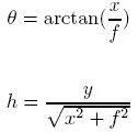
The scripts are:The first stage of the process was to warp all images into cylindrical coordinates. The output image is in (theta, h) coordinates, instead of (x,y). For each (theta,h) coordinate pair in the output image, an (x,y) coordinate pair was calculated from the original image, and its pixel value copied into the warped image using the following formulas:
Since the transformation from one coordinate space to another can result in non-inegral coordinates, some interpolation is necessary. This is done by taking the difference between the computed coordinates and their rounded values, and using these fractions as weights between the pixel at the rounded coordinates, and its neighbors, and a weighted average is taken of the 4 pixels in the neighborhood of the computed coordinates.
Once the images have been warped, I used the Sift Demo program released by David Lowe to exetract features from the images. Each feature consists of a coordinate in the image, a scale, and an orientation, plus 128 byte values summarizing the neighborhood of the feature. Using arc distance (which at small angles approximates Euclidean distance) as a similarity metric, features in one image were matched to features in another image. Then, using the RANSAC algorithm, outlier matches were discarded, and a homography was computed from the best matching feature pairs. This homography only consisted of translation and scaling terms, because the images were taken from a rotating platform, meaning that the only difference between images was rotational, which in cylindrical coordinates is a translation.
Stitching was accomplished by first finding the coordinates of the furthest image, then using its corners to find a bounding box. Then for every pixel in the output image, the coordinates in the frame of each source image were found. If the coordinates were inside the image, then the pixel from the original image was given a weight, and added to the output image. As in warping, the itransformed pixel coordinates are in general non-integral, so a weighting scheme among neighbors was used. Finally, the pixel value in the mosaic was divided by the sum of the weights of pixels matching its same location. The weights were based on the distance of each pixel in the source image from its center, divided by the distance from the center to the corners, so that the weights are in a [0 1] range.
Once the mosaic has been assembled, it has to be rotated (to counteract drift,) and cropped so that its edges form a rectangle with no empty areas in it. The vertical distance between the top of the first image and the top of the last image, divided by the width of the mosaic gives the tangent of the angle that the mosaic was rotated. Using that angle, a rotation matrix is assembled, and used to rotate the pixel coordinates of the mosaic to the new cropped image. Since there would still be a jagged edge at the top and bottom, a vertical margin was calculated using the same angle of rotation and the width of a single image, which gave the vertical range of that jagged edge, and the cropped image's size was adjusted accordingly.
While doing the image warping, an important detail is that while (x,y) coordinates have their origin at the upper left corner of the image, (h,theta) coordinates must have their origin at the center of the image because that is effectively the center or warping. If they are not calculated from the center, then the warping effect will not be centered in the image, resulting in un-matchable images.
In the matching phase, I found that if I computed homographies with rotation and shear terms included, that there was a slight bias towards compressing the top of the image, which causes an upward curvature on mosaics because successively compounded homographies would additively compound this effect, until images at the far end of the mosaic would be nearly vertical. One possible explanation for this is that the best fit is computed in a least squares sense, and if the coordinates are not normalized to a [0, 1] range, then large coordinates can be given far more weight than smaller ones, which could have the effect that coordinates at the bottom of the image would be matched more accurately at the expense of accuracy of coordinates at the top.
Some of the images taken could not be reasonably matched, because the features present were too regular. For instance, one sequence of images was of a hallway with bricks in a rectangular grid, and ceiling lights which also repeated down the hall, which resulted in a few very bad homographies in the sequence.
When using Matlab, it is very important to find out which operations take the longest to perform. By changing the array structed used by my stitching script to store all of the images in the sequence, I reduced the running time of the process from over 10 hours to under 10 minutes.