CS766 HW2
Yan Cao
Project 2 Report
Implementation steps
1. I
created a java class called ��CylindricalConvertion.java�� to convert the example
images to cylindrical views (saved as cXX.jpg). The central idea is realized by
this part:
for(int i=0;i<newWidth;i++){
for(int j=0;j<newHeight;j++){
double newX=focus*Math.tan((i-newOriginx)/focus)+xc;
double
newY=Math.sqrt((newX-xc)*(newX-xc)+focus*focus)*(j-newOriginy)/focus+yc;
int
nearestX=Math.round((float)newX);
int nearestY=Math.round((float)newY);
bufferedImage.setRGB(i,j,originalImg.getRGB(nearestX,nearestY));
}
}
2. I
used SIFTwin32 to generate key files (cXX.key).
3. Class
��FeaturePairFinder.java�� is used to find paired features between two photos.
Because in the key files generated from SIFT, each feature point is described
by a 128-dimention vector, for each point i
in one graph, I used kNN (k=2) to find the 2 closest points (j, k), then I used ��distance(i,j)/distance(j,k)>some cut value�� to get the candidate
pairs. It is realized by the function getPairs()
in this class. The feature pairs are saved in a vector with the following
format: ��Xnode1 Ynode1 Xnode2 Ynode2��
4.
RANSAC method is applied to get H between two adjacent graphs (m, n) so that
the new coordinates of n can be got by doing the multiplication
 (1)
(1)
]T.
The RANSAC is realized by the function getBestH() in class ��Ransac.java��. So if
we have N graphs, we get N H��s: H12, H23, ��, HN-1,N,
HN,1. Because we want to merge the N graphs to one
graph, we need to get H12, H13, H14, ��, H1,N,
H1,1 so that we can convert the other graphs��
coordinates to graph 1��s coordinate system. Here H1i
can be attained by using the following formula:
H1i= H12* H23*��*Hi-1,i (2)
Thus,
for graphs from 2 to N, use Equation 1 to do the transformation.
5. To
make the centers of the first graph and the last graph on a horizontal line, I
used a function shftY() to get a shift matrix S, where a=(centerY of the last
graph - centerY of the first graph)/ (centerX of the last graph �C centerX of
the first graph). Then update H1i to S* H1i

6. Calculate
the coordinates of the 4 corner points for each graph. Compare them and get the
minX, minY, maxX, maxY. The width of the new graph will be (maxX-minX) and the
height is (maxY-minY). Then shift the coordinate by using x=x-minX, y=y-minY,
so that the left top point moves to (0,0).
7. For
each pixel (x��, y��) in the new graph, calculate the coordinates in all the
original graphs by using
 , and then judge if it is in the ranges
of the original graphs. If in the range, pick the nearest pixel��s RGB value.
, and then judge if it is in the ranges
of the original graphs. If in the range, pick the nearest pixel��s RGB value.
8.
Blending. For each row i in the new
graph, I used 2 arrays to save the RGB values. These 2 arrays are initiated
with 0��s. If a pixel (i, j) is found in some graph, check if the jth element in
the first array rgb1[j] == 0, if true, set rgb value to it, if not, set rgb to
the jth element in the second array rgb2[j]. Then all overlapped parts can be
found in the second array because they are split by 0��s. Then find each
overlapped part and use feathering function a*rgb1[j]+(1-a)*rgb2[j] to get the
blended rgb.
Results
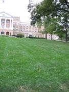
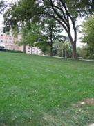
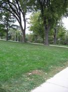
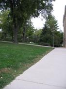
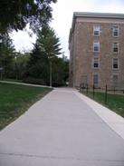
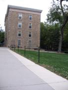
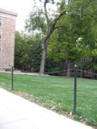
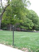
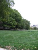
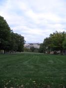
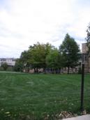
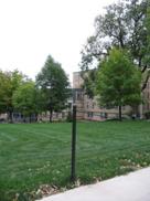
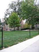
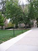
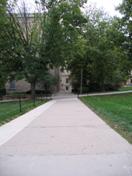
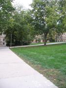
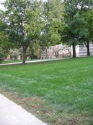
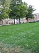
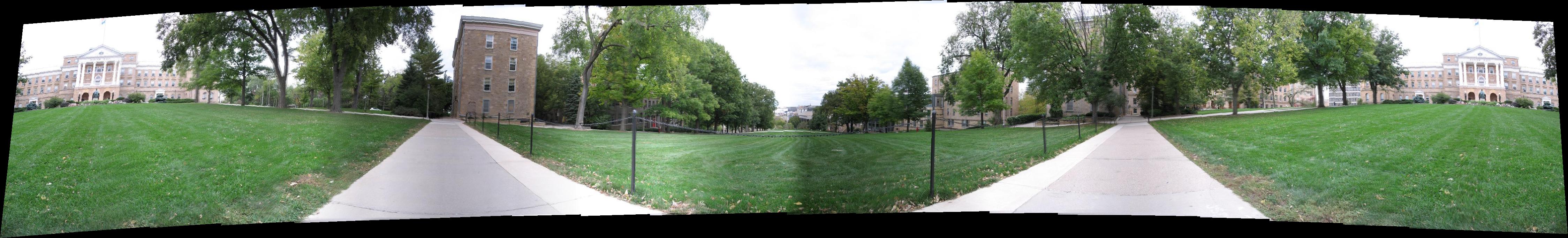
1.
Photos
taken by me in front of the Bascom Hall.


The panorama graph
generated (click to see full version):
The
graph is also shown in pano viewer.
2.
The
original graphs are the test graphs shown as following.
![]()
![]()
![]()
![]()
![]()
![]()
![]()
![]()
![]()
![]()
![]()
![]()
![]()
![]()
![]()
![]()
![]()
![]()
The
panorama graph generated (click to see full version):
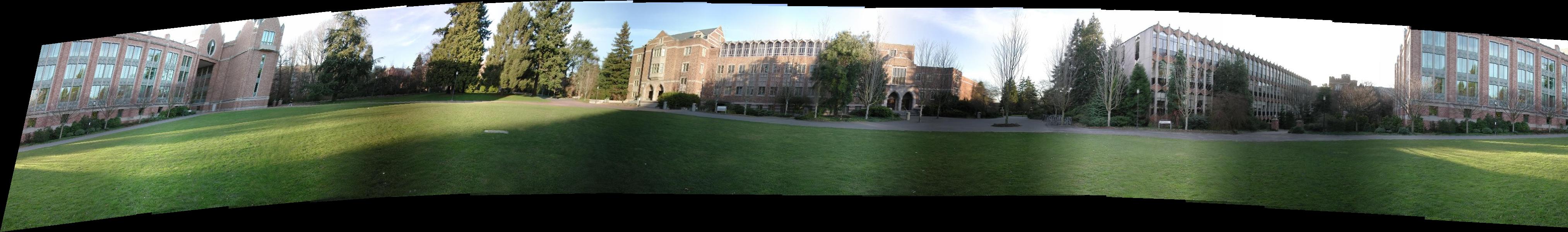
The
graph is shown in pano viewer.
Discussion
From the
result, we can clearly see the left part is obviously sheared. I think that it
might be caused by the accumulative stitching. Notice that there are 19 graphs
in total and the H for the19th graph is attained from a long
multiplication, H12* H23*��*H18,19.
So small values in positions (1,2) and (2,1) in H12, H23��. will cause big
values in H1,19.
The good
part is that I got a good result of feature match by using RANSAC. The
overlapped parts are perfectly stitched. I got it by trying different
parameters such as recursion times of RANSAC, cut value of feature pairs in
feature selection(see step 3 in the first part).
Appended Discussion
I first
generated the panorama from the sample graphs. I found there is a significant
shear effect at the end of the panorama. Thus, I decide to change my algorithm
a little bit to see if it can be solved in my new photos. Instead of using the
coordinate system of the 1st graph, I choose the coordinate system
of the graph in the middle. Since I have 20 consecutive photos (if we see the
first one also the last one, we have 21 in total), I use the 11th
graph as the basis, and transform the graphs on its left and right. From the
result, we can see the shear effect is somewhats weakened.