Project 1 High Dynamic Range Images
Shengqi Zhu,
Yancan Huang, Jiasi Song
Two kinds of Image Assignment Algorithms are done by Jiasi Song.
Basic HDR algorithm and the other HDR algorithm are done by Shenqi Zhu.
Tone Mapping algorithm is done by Yancan Huang.
Content
Comparison
of Tone Mapping Results
Summary of Bonus Points
In addition
to basic requirements, we have implemented 4 bonus: 2 image alignment
algorithms, 1 additional HDR algorithm and 1 tone mapping algorithm.
Input
Put all
the input data in one txt file, like input.txt. Then execute the exe file with
the directory name containing “input.txt” as the first argument.
The
first line of the input file is N, which is the number of images.
Then
following N Lines, each line has an image name(including path) & image
exposure time.
In the
(N+2)th line, there is a number indicating which alignment method you choose, 1
or 2 or 0.
If you
choose 1, the next line will be one integer parameter (moveRange, the value of
which depends on the image size and the translation length, the more the ratio
of the image’s translation distance to its size, the less the parameter you
input, the recommended value is 20 for a slightly misaligned group of images)
If you
choose 2, you have to input 2 integer parameters, BinNum(the recommended value
is 64) and moveRange(the same as method 1).
The next
line designates the method of HDR.
Similarly, put 1 here indicating method 1 and 2 here indicating method
2.
If you
choose 0, the image alignment will not be executed.
Method 1
of HDR needs 2 parameters: the number of pixels used for calculation (usually 100),
and the lambda parameter indicating how smooth the curve should be (5 will do
good).
Method 2
of HDR also needs 2 parameters: the number of pixels used for calculation
(usually 1000) and the epsilon for the termination criteria (usually 0.01)
Input.txt
for instance:
5
Image1.jpg
0.1
Image2.jpg 0.2
Image3.jpg 0.4
Image4.jpg 0.8
Image5.jpg 1.6
1 <-
indicating Method 1 of Image Alignment
40 <-
indicating parameters for Method 1
2 <-
indicating Method 2 of HDR
100 5 <- indicating parameters for Method 2
The
result.hdr will be in the same directory as the program argument.
Algorithms
Image Alignment
Two
methods in our project are done to do image alignment:
Ward's MTB algorithm
This
paper converts normal images to bi-level images and use image pyramid to do
alignment.
Mutual Information
Metric
This is a
traditional way to do image registration. The mutual information (MI) [1] of
two images is from the concept of information theory and expresses how much the
information image A contains about image B, which combines both the separate
and the joint entropy values of the images:

The advantage of
MI is that even the gray values of two images are not in the same range, it
works well in image registration.
Test Results of
2 methods
Results of 2
methods using images with size 415*260:
|
|
Translation Before Alignment |
Alignment Results of
MoveRange 10 |
Alignment Results of
MoveRange 20 |
Alignment Results of
MoveRange 30 |
|||
|
Method 1 |
Method 2 |
Method 1 |
Method 2 |
Method 1 |
Method 2 |
||
|
Image1 |
(-7,-18) |
(-11, 47) |
(-7,-18) |
(-7,-18) |
(-7,-18) |
(-7,-18) |
(-6,-18) |
|
Image2 |
(0, 0) |
(0,0) |
(0, 0) |
(0,0) |
(0, 0) |
(0,0) |
(0, 0) |
|
Image3 |
(-22, -4) |
(-22,-4) |
(-22, -4) |
(-22,-4) |
(-22, -4) |
(-22, -4) |
(-22, -4) |
The method 2 is
slightly faster and more robust than method 1.
HDR Generation
In
our program, we implement 2 different HDR algorithms, which show different
results.
Method 1
Implementation
Details
The
first algorithm is based on Debevec and Malik’s paper, but we made a few
changes. Debevec’s idea is that
each color channel can represent only 256 different values, so they only have
to find the correlations between measured brightness and irradiance with
respect to these 256 values. They
used photos with different exposure times and took advantage of the
characteristics of smooth curves to find the relationships. The fundamental of this algorithm is to
solve an overdetermined linear equation to get the result of least square error
estimation, that is, to do the following optimizations
![]()
In
our particular implementation, we have to settle down several things. First of all, since we don’t have to use
all the pixels on the images to calculate the relationship, how do we choose
points from the images? Basically,
we have to choose points that cover a wide range of scales (that is, let ![]() covers
from 0 to 255). Also, we don’t want
to choose points that change sharply in the image, since those points are most
likely to be random noises.
Therefore in our project, we tried two different ways of point
choosing. The first method is just
choosing points randomly from the image.
The second method takes account of the wide spread of the color. It first calculates the “expected values”
of the colors based on how many points we want to sample. Then it scans every point of the image
to find the most suitable point that is closest to the “expected values”. We have tried both methods, and the
final HDR image seems to have only slightly difference.
covers
from 0 to 255). Also, we don’t want
to choose points that change sharply in the image, since those points are most
likely to be random noises.
Therefore in our project, we tried two different ways of point
choosing. The first method is just
choosing points randomly from the image.
The second method takes account of the wide spread of the color. It first calculates the “expected values”
of the colors based on how many points we want to sample. Then it scans every point of the image
to find the most suitable point that is closest to the “expected values”. We have tried both methods, and the
final HDR image seems to have only slightly difference.
Another
change in our implementation is that we modify the weighting function. The original weighting function is

So
the “pure white” pixel (which intensity value is 0) and “pure black” pixel
(which intensity value is 1) accounts for no weight. So determining their irradiance will
rely fully on the smoothness of the curve, which will cause some flaws in the
image, as shown in the following figure.
One way to solve this problem is simply to add weight for black and
white pixels. In our
implementation, we use the following weighting function

It
gives us a better result which does not have substantial flaws, as shown in the
following figure.

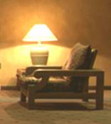
Figure
1 Final HDR image
using different weighting function.
Left image shows the original weighting function. Right image shows the modified weighting
function. See the difference in
bright areas.
Result
Our
first approach generates the following response curve using one of our camera
result.
Method 2
Implementation
Details
Our
second implementation follows the Mitsunaga and Nayar’s paper, but also made
several modifications. Their
approach does not need accurate exposure time as the first approach, and could
actually iteratively compute the exposure time. Their method assumes that the response
curve can be modeled using a high-ordered polynomial as
![]()
Their
approach is also optimizing the error function

However,
we made several modifications.
First, we assume that a measurement of 0 (black) should be mapped to the
irradiance of 0, and a measurement of 255 (white) should be mapped to the irradiance
of I(max). Therefore, we do not
consider the ![]() item, and
make it equals to 0. Second, we add
modifications to the calculation of the ration of two exposures R. The original formula is
item, and
make it equals to 0. Second, we add
modifications to the calculation of the ration of two exposures R. The original formula is

Note
that the original paper seemed to have a typo: it missed the 1/P fraction. Since the noise point could in fact interfere
with the iteration of R, and because images are assumed to have been sorted
from darkest to brightest, here, we take only ![]() to
calculate the R. It gives us a more
accurate result.
to
calculate the R. It gives us a more
accurate result.
Results
We
use the same group of pictures to test this method, and it gives us the
following response curve. The curve
is a 7-order polynomial function.
It is different from the previous method in that it does not make use of
the exposure time information which was given in method 1.
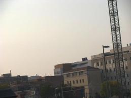
Here
is the comparison between these two methods. Since they only give the relative irradiance
value, the absolute exposure time is adjusted so that they look similar. As can be seen from the figure below,
method 1 seems to get a better image in that it generates more vivid color and
more specific details. But method 2
also has its own advantage, because it does not need exposure time
parameter.

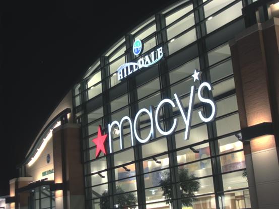
Figure
2 The generated HDR
image by 2 methods. Upper image is
using method 1 and lower image is using method 2.
Tone Mapping
In
this project, we implemented Tumblin’s LCIS Tone Mapping algorithm (Please refer
to their SIGGRAPH 1999 paper) as another Bonus Point. We applied both Tumblin’s
method and Reinhard’s approach onto the radiance map generated in the previous
step, and we compared the final result and draw some conclusions about the pros
and cons of these two tone mapping algorithms.
LCIS Tone Mapping
Approach
The
idea of LCIS Tone Mapping approach is analogized from the field of sketch
drawing: skilled artists preserve the details by drawing scene contents in
coarse-to-fine order using a hierarchy of scene boundaries and shadings. In
their SIGGRAPH 1999 paper, the authors proposed to build a similar hierarchy
using multiple instances of a new Low Curvature Image Simplifier (LCIS), a
partial differential equation inspired by anisotropic diffusion. Each LCIS
reduces the scene to many smooth regions that are bounded by sharp gradient
discontinuities, and a single parameter K chosen for each LCIS controls region
size and boundary complexity. With a few chosen K values, LCIS makes a set of
progressively simpler images, and image differences form a hierarchy of
increasingly important details, boundaries and large features. With this
method, we can construct a high detail, low contrast display image from this
hierarchy by compressing only the large features, then adding back all small
details.
We
summarize this algorithm as the following pseudo code which might be more
understandable than the description in the paper:
|
For each channel of Input
Image { Copy the current channel of Input
image into Temp image For each timestep {// Processing the Temp image once
and once again For
each link between neighbor pixels { Compute
the “curvature” at that link; if
this curvature is greater than some threshold mark
this link as boundary link and the two pixels as boundary pixels; } For
each pixel { if
not boundary pixel Compute
and apply flux through all corresponding links } } Copy the current channel of the
processed Temp image into Result image } |
Implementation Details
In
this project, we read carefully through the SIGGRAPH 1999 paper and referred
the source code fragment provided by the author, and finally implemented the
whole algorithm by our own.
Our
code is written is C++. We included the provided gil library to help process
the reading and writing of image files.
The
main function in our code takes several parameters which controls the effect of
our program:
float m_diffusKval: coductance
threshold
float m_diffusTstep: timestep
length
int m_diffusCount: number of
timesteps to run
bool m_diffusLeakfix: whether or
not enable the leakfix
By
trial and error, we found m_diffusKval from 0.001 to 0.01 and 200~800 timesteps
and leakfix enabled can produce best toning results.
Comparison of Tone
Mapping Results
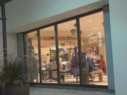
In
this part, we compare the tone mapping result of LCIS algorithm (in the left
column) and Reihard’s algorithm (in the right column).

(m_diffusKval=0.01,
m_diffusTstep=1, m_diffusCount=200, m_diffusLeakfix=true)

(m_diffusKval=0.001,
m_diffusTstep=1, m_diffusCount=200, m_diffusLeakfix=true)


(m_diffusKval=0.001,
m_diffusTstep=1, m_diffusCount=200, m_diffusLeakfix=true)


(m_diffusKval=0.01,
m_diffusTstep=1, m_diffusCount=200, m_diffusLeakfix=true)


(m_diffusKval=0.01,
m_diffusTstep=1, m_diffusCount=200, m_diffusLeakfix=true)
From
this comparison, we can easily see that the effect of LCIS is much poorer than
that of Reinhard’s algorithm, especially a dark halo around a bright object. On the other side, LCIS methods keeps
some details of the image much better, for example, considering the tree
feature in the last group of images above.
In
fact, based on LCIS, Raanan Fattal proposed a new HDR compression algorithm in
his SIGGRAPH 2002 paper in which he also compared the tone mapping result of
his algorithm vs. LCIS. Through comparison, he also pointed the problem of halo which proved our observation here.
[References]
1. F.MAES,D.VANDERMEULEN,ANDP.SUETENS,
"Medical Image Registration Using Mutual Information", IEEE
Transactions on Proceedings , Vol. 91(10), October 2003
2. Paul
E. Debevec, Jitendra Malik,
Recovering High Dynamic Range Radiance Maps from Photographs, SIGGRAPH
1997.
3. Tomoo
Mitsunaga, Shree Nayar, Radiometric
Self Calibration, CVPR 1999.
4.
Jack Tumblin, Greg Turk, LCIS: A Boundary Hierarchy for Detail-Preserving
Contrast Reduction, SIGGRAPH 1999.
5.
Raanan Fattal, Dani Lischinski, Michael Werman, Gradient Domain High Dynamic
Range Compression, SIGGRAPH 2002.
6.
Erik Reinhard, Michael Stark, Peter Shirley, Jim Ferwerda, Photographics Tone
Reproduction for Digital Images, SIGGRAPH 2002.