CS 766 Project 2: Panoramic Mosaic Stitching
Jiasi Song,
Shengqi Zhu, Yancan Huang,
We took
pictures, read references and discussed algorithms all together. Yancan
implemented step2, Shengqi implemented step3 and de-ghosted routine and Jiasi
finished step4 and step5.
Step 2: Warping to
Cylindrical Coordinates
Step3. Computing the
alignment of the images in pairs
BONUS: Ghost image
elimination
Step 4. Stitching and cropping
the resulting aligned images
Step 5.Creating the final
results
Summary of Bonus Points
In
addition to basic requirements, we have also implemented one bonus: Ghost Image
Elimination.
Input & Output
This program was developed under Matlab. To use this program, you should try to compile SIFT library first. Note that for different version of Matlab, you have to compile the library before the first time you use.
1.
To
Compile the SIFT library:
cd <Code Directory>
sift_compile()
2.
To
Run the code
cd <Code Directory>
panorama(<Pattern>, <StartPic>, <EndPic>)
Note: <Pattern> means the pattern of the filename series,
<StartPic> means the start number of the image, <EndPic> means the
end number of the image
For example, if you have a series of image like: data/IMG_0001.JPG,
data/IMG_0002.JPG, …, data/ IMG_0018.JPG, then your <Pattern> should be
‘data/IMG_%04d.JPG’, your <StartPic> should be 1, your <EndPic>
should be 18.
3.
To
Use de-ghosted Routine
Uncommented the line: img=step4_2(img, translation); in the panorama.m
and run panorama again.
The program will output its result as “result.bmp” in the code directory, and also shows the result on the screen.
Step 2: Warping to Cylindrical Coordinates
In this
step, we computed the mapping original images from plane coordinates to
cylindrical coordinates as the lecture slides showed. We have implemented two
versions of warping, one is Basic Warping and the other is Distortion-Free
Warping.
1. Basic Warping
Given
coordinate![]() in the original image, of which the height and width is
supposed to be
in the original image, of which the height and width is
supposed to be ![]() and
and ![]() respectively, the
corresponding cylindrical coordinates are:
respectively, the
corresponding cylindrical coordinates are:
 ,
,  .
.
We have
to guarantee that all![]() , thus we set:
, thus we set:
 ,
, 
Then we
have:
 ,
, ,
,
Therefore
we have the inverse mapping from cylindrical coordinates to original
coordinates:
 ,
, ,
,
According
to the mapping above and Bilinear
Interpolation, we can simply fill each pixel with weighted sum of values of
the neighboring pixels of coordinate![]() in the original image:
in the original image:
Suppose
the horizontal and vertical distances of position![]() with the left-top pixel are
with the left-top pixel are ![]() and respectively,
then we have:
and respectively,
then we have:
 .
.
2. Distortion-Free Warping
In addition
to basic warping, we have implemented the distortion-free warping algorithm
which aims to remove the edge effect of the lens.
As the
lecture slides showed, given pixel![]() , suppose
, suppose  , and
, and  , then we have:
![]() ,
,
![]() .
.
Since it
is difficult to get the analytic expression of ![]() in form of
in form of ![]() compared to part
1, so we resorted to another way: to “diffuse” the value of position
compared to part
1, so we resorted to another way: to “diffuse” the value of position ![]() to its
neighboring pixels with the weight similar as part 1.
to its
neighboring pixels with the weight similar as part 1.
For
example, the left-top pixel is contributed by position![]() with value of
with value of ![]() , the left-bottom pixel is contributed with value of
, the left-bottom pixel is contributed with value of ![]() , the right-top pixel is contributed with value of
, the right-top pixel is contributed with value of ![]() , and the right-bottom pixel is contributed with value of
, and the right-bottom pixel is contributed with value of ![]() .
.
We tested
these two warping approaches with the sample images provided on the project
webpage and got some warped result images as follows (the top is the original
image, the lower left is the result of basic approach and the lower right is
the result of distortion-free approach):
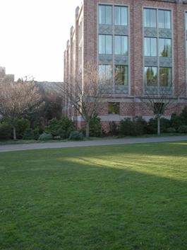
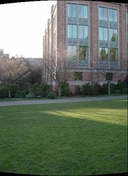
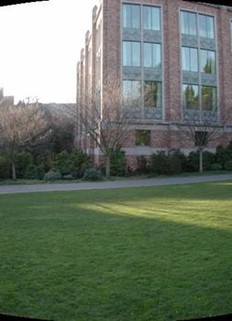
We can
see that in the border area of the result images, the distortion-free method
eliminates the edge distortion much better. In fact, such distortion affects
the following stage of this project, i.e. feature detection, quite a bit, so it
is very important to remove such distortion; thus in the final version of our
code we adopted the distortion-free warping approach.
Step3. Computing the alignment of the images in pairs
We used RANSAC algorithm to compute image alignment matrix. Here, since we already warped the image in step 2, we only consider the translational displacement.
The most important thing is to select features of two consecutive images and match these feature points. We used SIFT feature as was described on the class. Although there seems to be many other choices, SIFT is famous for its stability. We have tried different threshold for the distance of the matching routine, and in a very wide range the result is stable. However, there are two drawbacks of using SIFT. First, SIFT is relatively slow and memory-consuming compared to other simple features. Secondly, SIFT only makes use of gray scale information, but no color information is taken into consideration, which means when two features are similar in intensity but different in color, SIFT cannot differentiate them very well. Here, we used a Matlab implemented SIFT from http://vision.ucla.edu/~vedaldi/code/sift/sift.html.
RANSAC algorithm is not hard to implement. Here, we used a threshold of 2 pixels of distance between corresponding features to distinguish inliers and outliers. We also used the following images to test the algorithm, as shown in Figure 1. These two crosses are offset by 10 pixels in x and 10 pixels in y, with a little variant in the length and positions of two lines. SIFT successfully found the features of the image, as shown in Figure 2. And the RANSAC algorithm gave us a very ideal transform matrix: the x offset is exactly 10, while the y offset is 9.75, only with a 2.5% error.
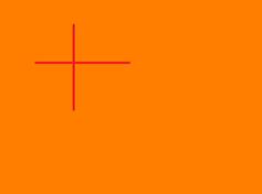
Figure 1 Test Image of RANSAC
Figure 2 Features found by SIFT
BONUS: Ghost image elimination
In our panorama, we purposefully added some moving objects, such as human beings, for demonstrating the ghost phenomenon. There are a few papers emphasizing on the elimination of ghost images, and here we modified and implemented one method. This algorithm is from Uyttendaele et al. However, in our experiment, when there will not be an overlapped area covered by three or more photos, we can simplify its implementation.
The main idea here is to search for regions
of difference (ROD) and then eliminate the contribution of ROD of inconsistent
images. For the searching process,
we first do it on pixel level, that is, calculate the difference of overlapped
images and mark the pixel as a “ghost pixel” if the difference is larger than a
threshold. The tricky part is how
to measure the difference. Surely
we can use ![]() to
represent the difference, it is somewhat inconsistent with our sense. A more proper way is to use gray scale
value, but light change will greatly affect the result. Another way is to use
to
represent the difference, it is somewhat inconsistent with our sense. A more proper way is to use gray scale
value, but light change will greatly affect the result. Another way is to use
Next, we combine these “ghost pixels” to form larger “ghost objects”. We use morphological transformations (erode and dilate) to combine pixels that are close to each other, and also to eliminate small noise points. After that, we use Connected Component Labeling to group connected pixels to form an object. This step allows us to operate image in a more high-level way.
As long as we get the Connected Component, we can eliminate one of the “ghost objects”. Which ghost object shall we choose is still a tricky problem. Empirically, objects that are more close to the center of the image are usually more reliable and have less distortion. So we calculate the distance from the object to the edge and find a more suitable winner. We simply eliminate the loser here for simplicity. But more suitable way is to do a cross fading around the edge.
The result of this ghost elimination is shown in Figure 3. For the purpose of comparison, we have shown both the ghosted image and the de-ghosted image. The result shows that some of the ghost area (face and right leg) was successfully removed, while some other areas (left leg) was not removed. This is probably because the pixels around the left leg do not have much differences in the two images, therefore, these pixels cannot be marked as “ghost pixels”. Figure 4 shows another example, see the difference of the vase.
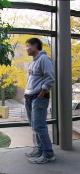
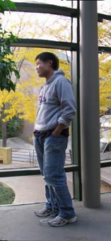
Figure 3 Ghosted Image (left) and De-ghosted Image (right)
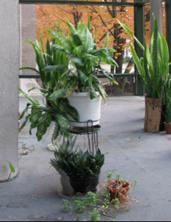

Figure 4 Another example of Ghosted Image (left) and De-ghosted Image (right)
However, such method will also bring about problems. Simply eliminate the weight of one image will cause some areas to be inhomogeneous, as shown in Figure 5. The flaw in the ceiling area clearly shows this drawback. One improvement method would be to do a cross fading around the edge.
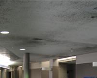

Figure 5 Flaw of De-ghosted Process, Ghosted Image (left) and De-ghosted Image (right)
Step 4. Stitching and cropping the resulting aligned images
The code
of this part is in “step4.m”, it has two arguments: images to be stitched and
matrixes of image alignment.
This
program implements the following functions:
1) Calculate
how large the final stitched image will be
2) Resample
each image to its final position;
To solve interpolation problem, the
inverse of transform matrix is used here, and we choose bilinear method [1] to
do image interpolation:
3) Blend
overlapped images
We used a weighting function:
Where PA, PB is
corresponding pixel value in overlapped images A and B, and dA (dB)
is the minimum distance from the pixel to the edge of Image A(B).
4) Make
the left and right seam perfectly, which has two steps:
A. Do
a linear wrap to remove vertical drift between the first and last image:
Y’=y+ax;
a=Δy*(x-x0)/(x1-x0)
B.
Shear the left and right end of the
image
5) Some
Results of blending:

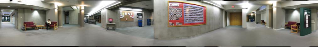
Step 5.Creating the final results
References
[1] http://en.wikipedia.org/wiki/Bilinear_interpolation
[2] R. Szeliski, H.-Y. Shum. Creating full view panoramic image mosaics and texture-mapped models, SIGGRAPH 1997, pp251-258.
[3] M. Brown, D. G. Lowe. Recognising Panoramas, ICCV 2003.