Project 3: Photometric Stereo
Ba-Quy Vuong and Nan Chen
In this project, we implemented a system to construct a height field from a series of images of a diffuse object under different point light sources. In addition to creating photometric stereos, we also implemented the following extensions:
Estimating light source directions and surface normals simultaneously: By using just a set of images of an object under different light source directions, we can construct both light source directions and surface normals without using the chrome ball.
Improving height estimation by using intensity weighting or smooth constraints: By incorporating the smoothness constraints in estimating height field, we can make the estimate more robust. Also, by giving different intensity different weight in the objective function, noises in extreme dark or bright area can be effectively removed.
2. The overall process
The process of constructing photometric stereos basically consists of four steps:
Light Source Direction Estimation: Using a chrome ball under different light source point, we can construct the directions of these light sources since the normal at any given point on the ball is known.
Surface Normal Estimation: After all the light source directions are determined, we can estimate the surface normal vectors of each point on the object.
Albedo Estimation: The albedo of the surface can be computed simultaneously with the surface normal or can be computed separately. In our implementation, we calculated them separately for better accuracy.
Height Estimation: After the surface normals have been calculated, we can compute the height of each image pixel. These heights give the depth of the image and thus help us to construct the 3D view of the object.
Light Source Direction Estimation:
First, we determine the center of the chrome ball by calculating the coordinates of its center in the mask image. The algorithm is straight forward, we just take the averages of X and Y coordinates of all the pixels belong to the ball in the mask.
Next, we determined the radius of the ball by taking the averaging distance from boundary pixels to the center.
Then, for each image of the chrome ball, we estimated the highlight center by taking the averages of X, Y coordinates of all the pixel in the highlight area. This is similar to determining ball center, except that we weighted each image by its intensity.
Finally we computed the light source direction using the formula
![]()
where N is the normal vector at the highlight center point and R is the reflection vector. R=(0,0,-1) and N is the normalized vector of (hx,hy,cx,cy are the coordinates of the highlight center and ball center respectively. r is the ball’s radius):
Normal Calculation:
The
appearance of diffuse objects is modeled as
![]() where
I is the pixel intensity, kd
is the albedo, and L
is the lighting direction (a unit vector), and n
is the unit surface normal. Let g=kdn,
g
can be calculated by solving a linear squares problem. The objective
function is:
where
I is the pixel intensity, kd
is the albedo, and L
is the lighting direction (a unit vector), and n
is the unit surface normal. Let g=kdn,
g
can be calculated by solving a linear squares problem. The objective
function is:
![]()
Once we have the vector g=kdn, n can be computed by normalizing g.
Abedo Calculation:
To make the estimates more accurate, we use another least square estimation after normal estimates. Basically, we find the albedo for each channel by minimizing
![]()
for the set of all images. The albedo can be solved analytically in the situation by
![]()
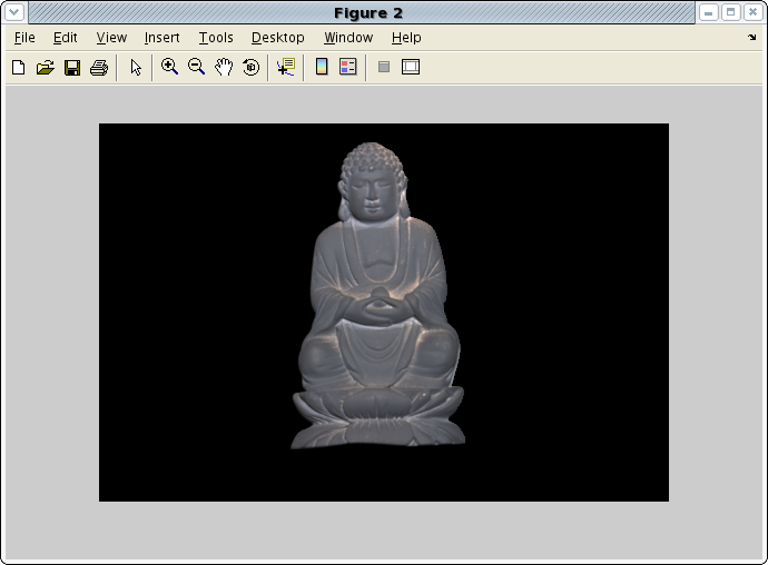
After we solve the albedo for each channel respectively, we can combine them into a RGB channel image, and display it accordingly. The results listed following indicates that albedo for different channel have close relationship with the color channel of the original images.
Height Estimation:
After normal vectors for each point are estimated, we can also estimate the height for different point by solving the equation array
![]() and
and
![]()
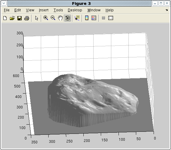
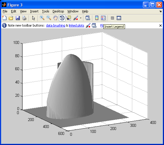
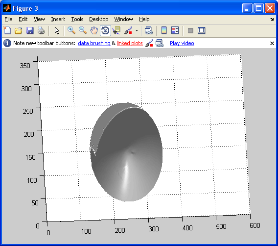
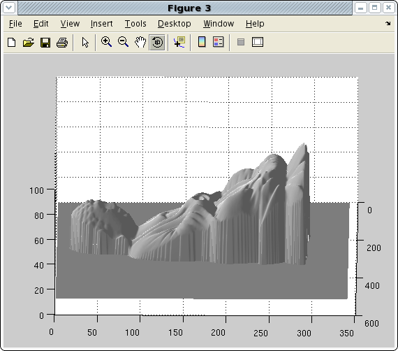
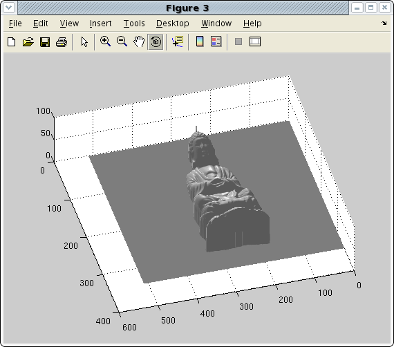
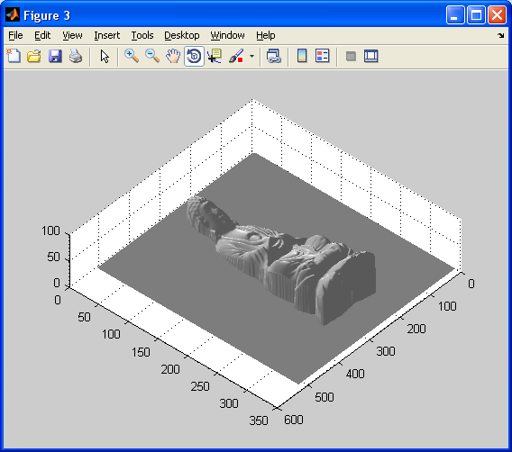
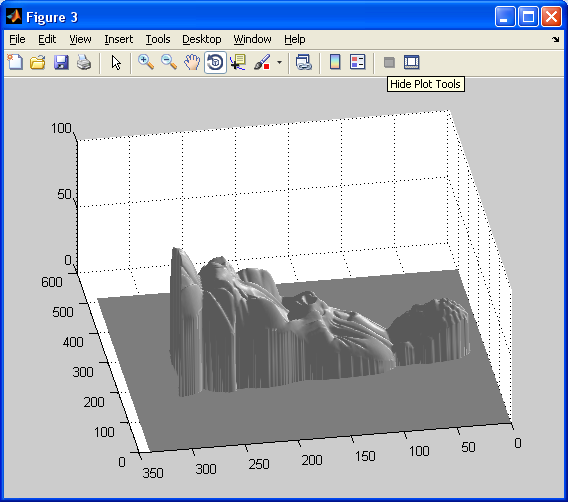
using least square methods. Because of the sparse character of coefficient matrix, we use the sparse matrix in Matlab to save memory in computation. After we estimate the height in the mask area, we can use surfl to plot the 3D shape and can view it from different angle. Detailed results are shown in the next section.
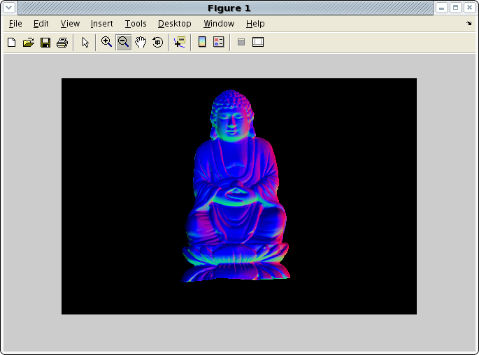
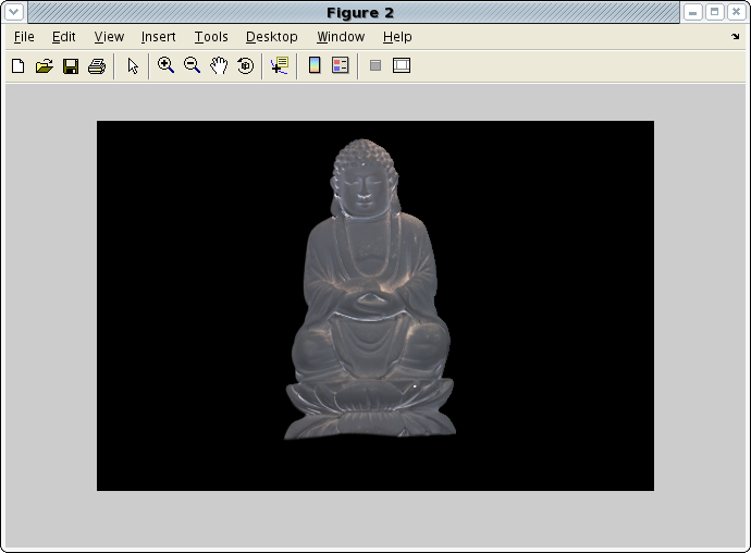
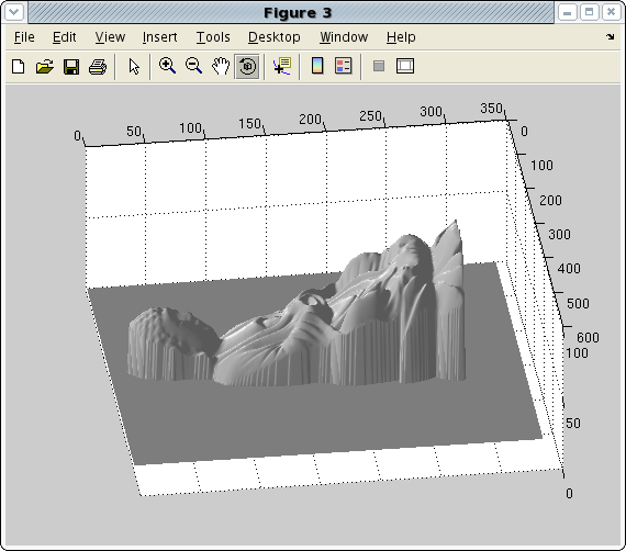
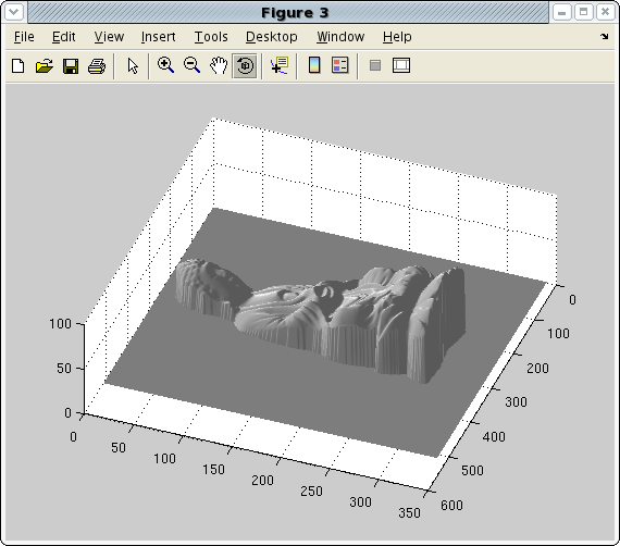
Buddha
|
|
|
|
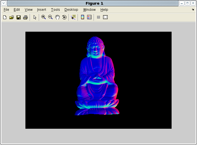
Figure 1: RGB-encoded normals |
Figure 2: Abedo map |
|
|
|
|
Figure 3: Reconstructed surface 1 |
Figure 4: Reconstructed surface 2 |
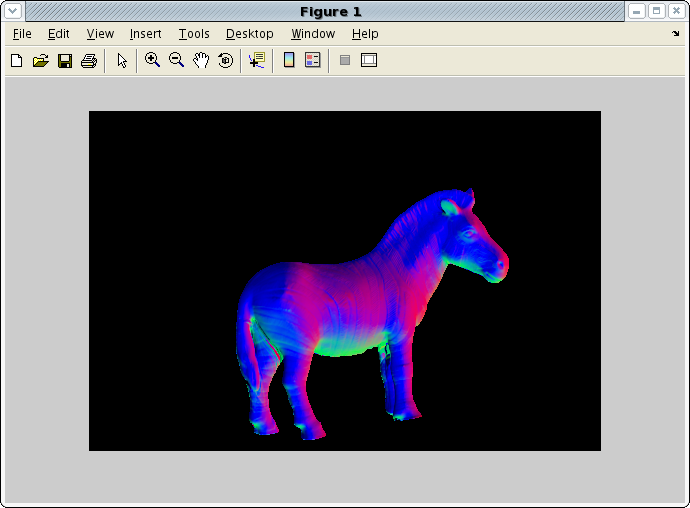
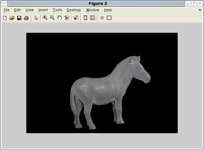
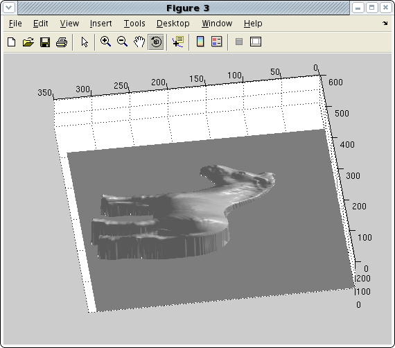
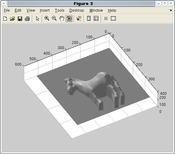
Horse
|
|
|
|
Figure 5: RGB-encoded normals |
Figure 6: Abedo map |
|
|
|
|
Figure 7: Reconstructed surface 1 |
Figure 8: Reconstructed surface 2 |
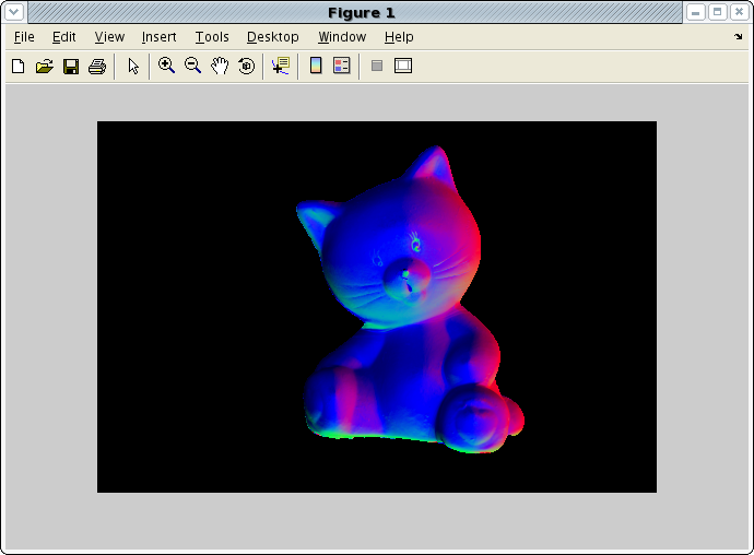
Cat
|
|
|
|
Figure 9: RGB-encoded normal |
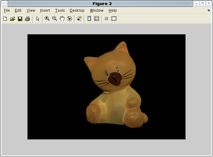
Figure 10: Abedo map |
|
|
|
|
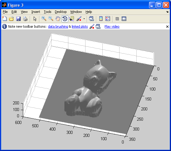
Figure 11: Reconstructed surface 1 |
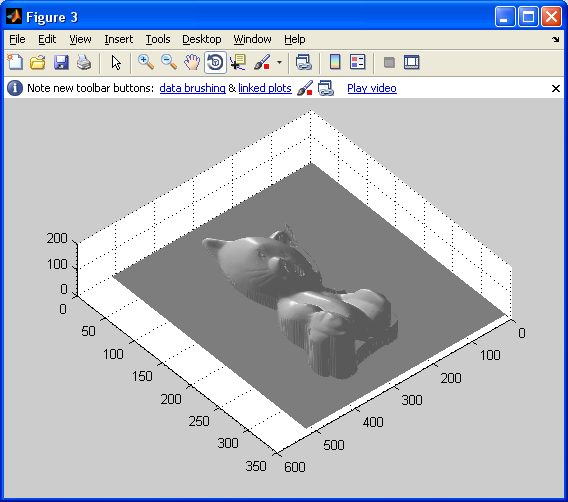
Figure 12: Reconstructed surface 2 |
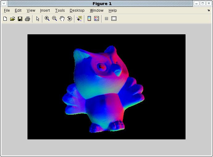
Owl
|
|
|
|
Figure 13: RGB-encoded normals |
Figure 14: Abedo map |
|
|
|
|
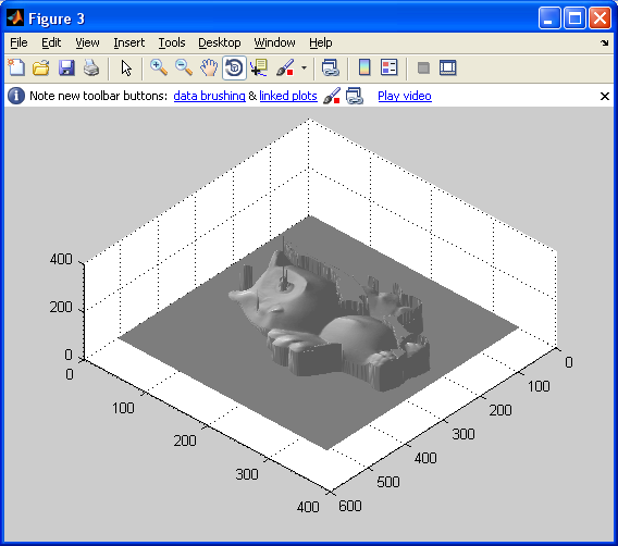
Figure 15: Reconstructed surface 1 |
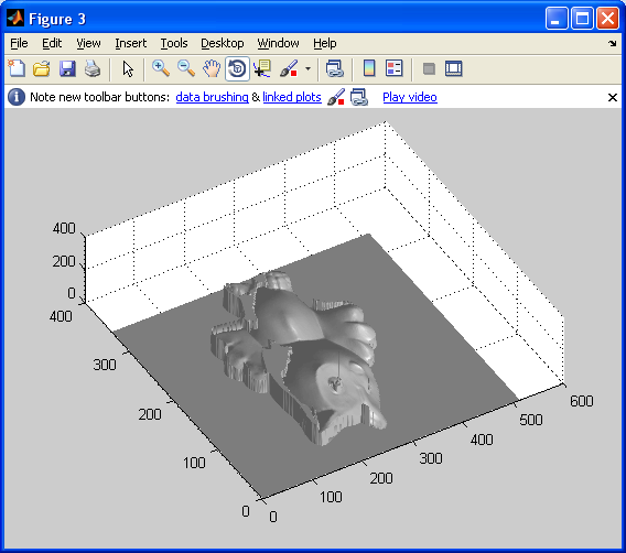
Figure 16: Reconstructed surface 2 |
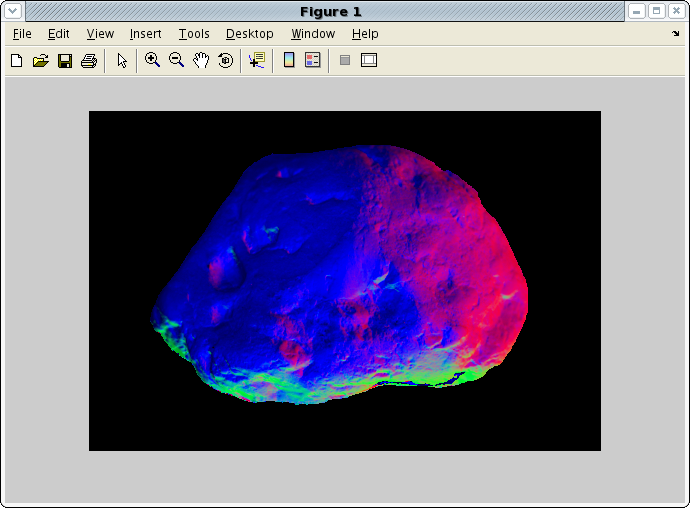
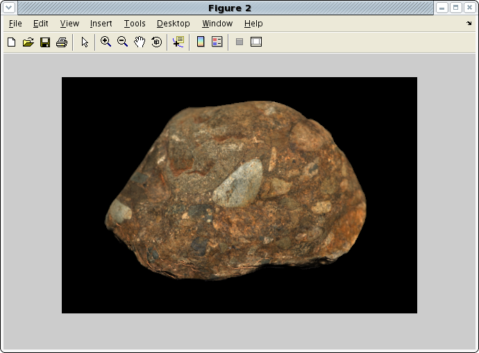
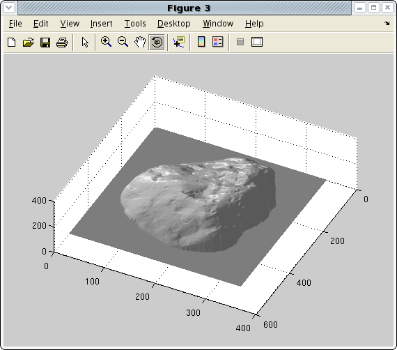
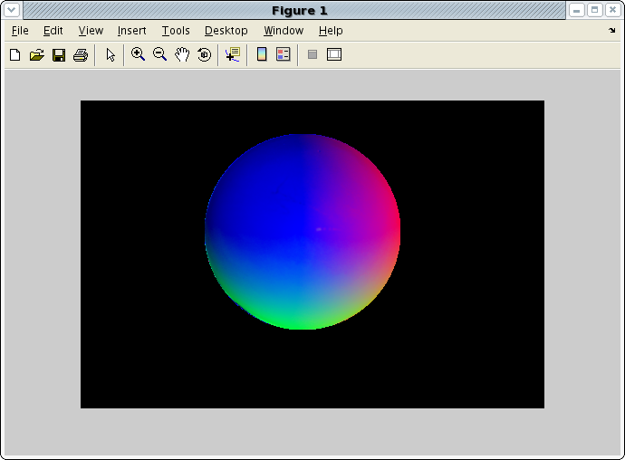
Rock
|
|
|
|
Figure 17: RGB-encoded normals |
Figure 18: Abedo map |
|
|
|
|
Figure 19: Reconstructed surface 1 |
Figure 20: Reconstructed surface 2 |
Gray
|
|
|
|
Figure 21: RGB-encoded normals |
Figure 22: Abedo map |
|
|
|
|
Figure 23: Reconstructed surface 1 |
Figure 24: Reconstructed surface 2 |
This algorithm estimates the light source directions and surface normals simultaneously. Thus, a separate step of estimating light source direction is not needed. The algorithm works as follows.
First, the Image Data Matrix I is constructed. Assume there are f images, each has p pixels, then the matrix I is
where iij is pixel intensity.
Next, using SVD we have I=U∑V. Let U’, ∑’, V’ be the sub-matrices of U,∑,V by taking the first 3 columns, first 3x3 matrix, and first 3 rows respectively.
Define
![]() and
and
![]() .
.
Compute
the matrix A such that
![]() where
p’ is the number of pixels that have the same surface reflectance.
where
p’ is the number of pixels that have the same surface reflectance.
Finally,
the normal is the normalized version of
![]() and
the light source direction is the normalized version of
and
the light source direction is the normalized version of
![]()
When implementing this algorithm, we realized that it is crucial to do coordinate transformation as the coordinates used by the algorithm are different from what we are using. After doing coordinate transformation, the result is very optimistic.
|
|
|
|
Figure 25: RGB-encoded normals using the simultaneous algorithm |
Figure 26: Abedo map using the simultaneous algorithm |
|
|
|
|
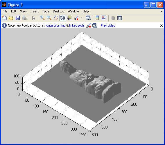
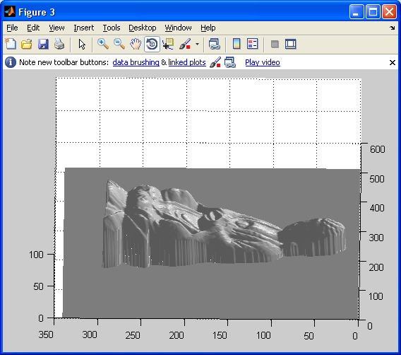
Figure 27: Reconstructed surface 1 using the simultaneous algorithm |
Figure 28: Reconstructed surface 2 using the simultaneous algorithm |
In previous sections, we estimate the height field by solving the following least square optimization problem
![]()
However, the solution to this function has some issues need to be resolved. First, the results may not be smooth enough for a surface. Second, the noise introduced in extreme dark or bright area may make the estimate of normal vectors inaccurate, and therefore make the estimate of height field unreliable.
Considering these two issues, we change the objective function to improve the estimate of the height field. Our first method adds a constraint term in the objective function to control the second order derivative not to be large. Specifically, we want to find
In the above equations, we use
![]() and
and
![]()
to approximate the second order derivative along x and y directions respectively. λ is the factor controlling the weight of the smooth constraints. The recovered height field with smooth constraints is shown in the following figure:
|
|
|
|
Figure 29: Reconstructed surface 1 using smooth constraint recovery |
Figure 30: Reconstructed surface 2 using smooth constraint recovery |
On the other hand, the pixel value close to 0 or 255 could not represent the real intensity well. Therefore, a intensity weighting method is necessary to effectively eliminates the noise. Therefore, we use the similar weighting as
![]()
And the corresponding objective function can be expressed as
![]()
where the intensity weighting comes into play to determine which constraint is more important for height recovery. The results is shown in the following figures:
|
|
|
|
Figure 31: Reconstructed surface 1 using intensity weighting |
Figure 32: Reconstructed surface 2 using intensity weighting |
From the results we listed above, we can find that our algorithm does not work for all the image set. One common observation among those failed images is that at some point, the normal vector estimation is not stable. In another world, we may get a matrix with rank less than 3, therefore, the obtained normal vector is misleading. We can find from the failed image that when there is some dark area, such as eye ball, or hair, the normal estimation would be inaccurate.
A possible solution to this is set a threshold of the image pixel value. When the pixel value is smaller than that, we can just ignore this pixel, and do not use its normal vector in estimation. However, if we just ignore these normal vectors, the corresponding height will have defects, and more sophisticated method should be used to get satisfactory results.
Our group has two members and the work was distributed as follows:
Ba-Quy Vuong
Light source direction estimation
Normal vector estimation
Extension: Estimate normal vectors without knowing light source directions
Nan Chen
Abedo estimation
Height calculation
Extension: Estimate height field with smooth constraints and intensity weighting
[1] Woodham, Optical Engineering, 1980, Photometric Stereo
[2] Hayakawa, Journal of the Optical Society of America, 1994, Photometric stereo under a light source with arbitrary motion
[3] Example-Based Photometric Stereo: Shape Reconstruction with General, Varying BRDFs A. Hertzmann, S. M. Seitz. IEEE Trans. PAMI. August 2005. Vol. 27, No. 8, pages 1254-1264.