Introduction
            The goal of this project is to reconstruct the three dimensional shape of an object which is view under a variety of lighting conditions.  The object is imaged using a single light source, which has been moved twelve times to provide twelve uniquely lighted images.  Using a reflective chrome sphere, the lighting directions can be calibrated for each of the twelve cases based on the location of highlights on the sphere.  With this calibration information, the surface normals of the object can be found based on pixel intensity over the twelve cases, from which a depth map can be found, giving the three dimensional structure of the object.
Algorithm

1. Image pre-processing
2. Calibration with chrome sphere
3. Solving surface normals
4. Solving for color albedo
5. Least squares surface fitting

1)    Image Pre-Processing
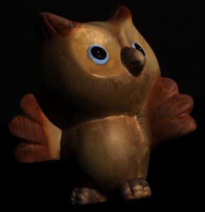
The provided images for this project are given in .tga format.  Matlab, the program used for this project, does not handle this image format, so the images needed to be converted to a usable form.  The Able Batch Converter was used to convert all of the images from .tga into .bmp format, which is an accepted image format in Matlab.

2) Calibration with chrome sphere
Calibration is performed on the chrome sphere to determine the light vectors for each of the twelve lighting cases.  The first step is to determine the parameters of the sphere, which are the centroid and the radius.  To do this, the mask image of the sphere, chrome.mask.tga, is used to create a binary image by thresholding the RGB image such that an intensity of 128 or above was assigned a 1, and any intensity below 128 was assigned a 0; this made the sphere white and the background black. From this binary image, the centroid of the sphere was calculated to be at (254.2, 148.7).  The radius of the sphere was found as the distance from the centroid to the edge of the sphere determined with a simple gradient calculation. The radius was found to be 120.1 pixels.

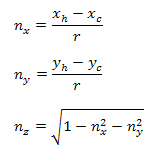
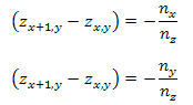
The lighting images of the chrome sphere were used to determine the light vectors. First the images were thresholded to form a binary image to isolate the highlight.  The centroid, (xh,yh) of the highlight was then found, which is where the light vector hits the sphere.  The surface normal unit vector at the centroid point is then found using the following equations:

At the location of a highlight, the reflected light, R, of the highlight is assumed perpendicular to the image sensor of the camera, which leads to the following geometric relationship:

Being perpendicular to the camera, R is defined as <0,0,1>.  This relationship allows us to solve for the lighting vector in each of the twelve cases.

3)    Solving surface normals
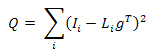
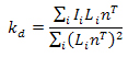
Knowing the lighting vectors in each case, we can find the surface normals for each pixel of the object.  Assuming a camera response function of 1 and a light source intensity of 1, the following equation relates the pixel intensity of a single color channel, I, to the lighting vector, L, albedo of the color channel, kd, and surface normal vector, n:

The unknowns in this equation, surface normal and albedo, are lumped into one term and substituted into the previous equation

The quantity g is then solved for byusing a least squares solution intended to minimize the objective function.

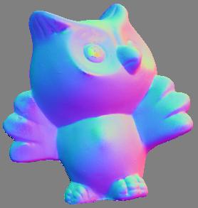
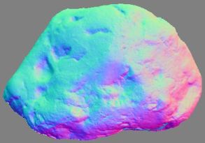
We can recover n by making g a unit vector, effectively dividing by kd.  Each color channel can provide a surface normal, so the normal used for the project image was derived from a grayscale of the image in an effort to “average” the RGB surface normals.

4)   Solving for color albedo
Now that the surface normal for each pixel is found, we need to determine the albedo at each pixel for each color channel.  We aim solve for the albedo which minimized the objective function:

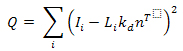
This is done by differentiating the objective function and solving for kd, giving the following equation to compute the albedo for each pixel.


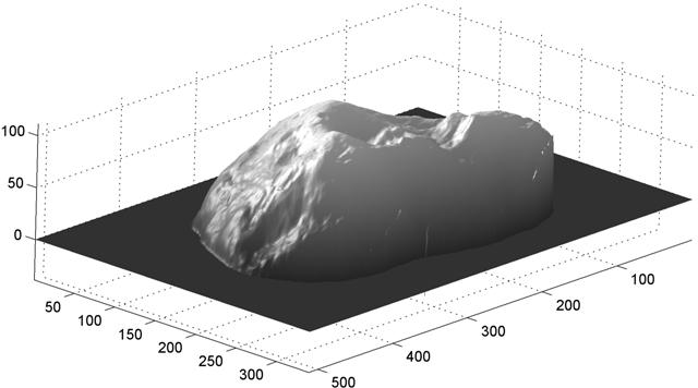
5)   Least squares surface fitting
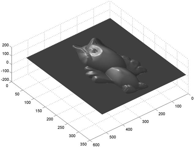
The surface normals give us knowledge of the curvature of the object’s surface and from this information, we can estimate the shape of the object.  First estimate a vector parallel to the surface at each pixel and thus, perpendicular to the surface normal.  To do this, we assume that a vector between two neighboring pixels is parallel to the surface, given by the following equations for both x and y directions.

Since the vectors vx and vy are both perpendicular to the normal, the dot product between each vector and the normal will zero, giving us the following relationships:

This relationship can be written in matrix format for every pixel on the object, giving:
Mz = v
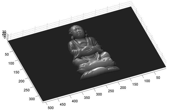
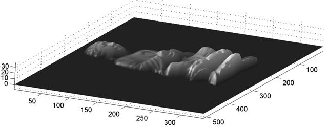
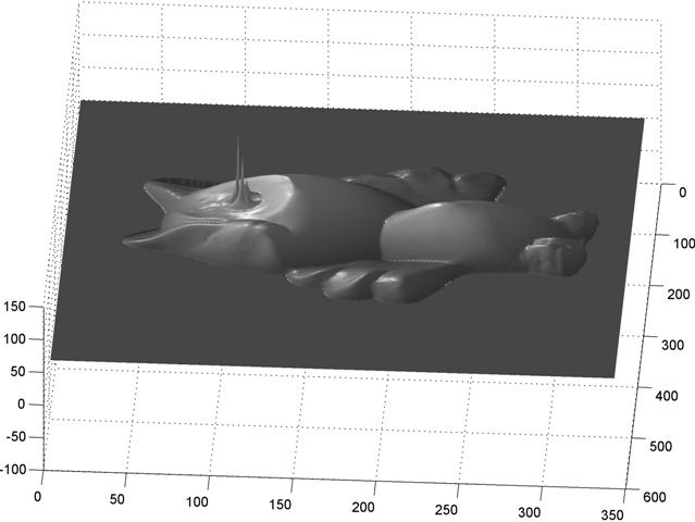
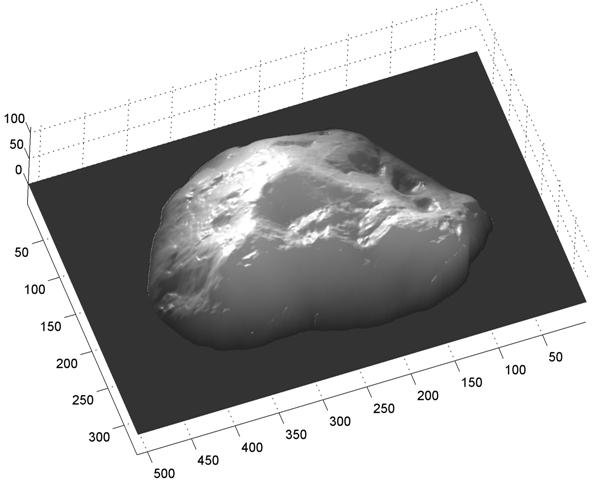
  However, the M matrix is very large; if n is the number of pixels on the object, the matrix is of dimension 2n-by-n.  For this reason, sparse matricies are utilized to store the information using less memory by omitting the zeros and only storing the actual data points.  The matrix equations are then solved for using a least squares solution, which provides the depth matrix of the object.
Implementation
The algorithm was implemented in MATLAB using these scripts:
calibration.m – Solves for the centroid and radius of the chrome sphere.  Solves for the lighting vectors of the chrome ball calibration images.
normal.m – Solves for the surface normal of the grayscale image.  Composes the RGB-encoded normal map
albedo.m – Solves for the albedo of each RGB color channel.  Composes the albedo map.
fit_surf.m – Solves for the depth matrix for the object using sparse matricies.

Results
            The algorithm was implemented on three images, Buddha, owl, and rock, with the results shown below.  Each image features the following results: an RGB-encoded normal map, an albedo map, and two 3-D views of the surface.

The first object, Buddha, matched the provided normal and albedo maps failry well. In addition, the surface fit appears to be reasonable compared to what is expected from the image.

	Buddha
Original image	Surface Normal Map	Albedo Map
Surface Maps

The second object, owl, also saw good results, except on the pupil of the eye, which is shown on the surface map as a collection of spikes. This is likely due to the fact the in the original images, the pupil is a black region, so when finding the normals, the solver was unable to resolve the region correctly. This is then reflected in the surfac map as incorrect depths.

	Owl
Original image	Surface Normal Map	Albedo Map
Surface Maps

	Rock
Original image	Surface Normal Map	Albedo Map
Surface Maps

Overall, I think the results of my algorithm are pretty good.

Discussion
This project seemed to give me the most problems of all of the projects so far.  One of the main issues I had was the numbering of the arrays in Matlab, as the y direction is flipped when using images.  This caused issues for me first with the lighting vectors being upside-down.  Then, when computing the surface plot, I ran into the same issue when programming in the M matrix, as the y neighboring pixel was actually above the pixel of interest in the matrix rather than below it as in the image. 
In addition, I ran into major issues trying to set up the M matrix.  At first, I tried to used every pixel in the image and got a surface map which made no sense.  I then tried to limit it to just pixels of the object, but still was unable to solve the depths correctly.  Finally, I realized that my programming of M was too simple and dictated some neighboring relationships that did not exist, which is why the depths were incorrectly solved.  With this issue resolved, I was finally able to achieve the surface map.
This method of recovering the surface map of the object is interesting and quite clever. However, at least in my case, the implementation was painful due to the very large matricies involved. When I ran into a problem, I could not look at the matrix I had created for any hints as to what the issue actually was, as the matrix was simply too huge. Now that I have a program written to do the analysis, I'm sure it would go a lot smoother the second time around.

Software Used
Matlab
Able Batch Converter