Outline

Introduction
Approach
Results
References

Introduction

Photometric stereo recovers depth information from multiple images under different lighting conditions.

Approach

Lighting Directions

The first step in our approach is to determine lighting directions from images of chrome balls. If we model these as purely specular, then it is a simple process to recover a light vector. The full process of recovering the vector is:

1. compute centroid and radius of chrome ball.
2. compute center of reflected light on the ball
3. the normal, N, at that point in the direction of the line extending to the centroid
4. assume that the viewing angle, A, is in a constant direction for all pixels.
5. the light direction then is 2 * (N * A') * N - A

Normals and albedo

Once we know the light directions, we can recover the normals at each pixel. If we assume a diffuse object, then the pixel intensity, I_i_k, for pixel i, image k, is given by I_i_k = kd_i * N_i * L_k'. We can solve for kd_i * N_i together, and then normalize the result to obtain our normal vector. That is we minimize
Q = Σ_k (I_k – L_k * g )^2
To minimize shadows and specular highlights we use a weighting function. Then our objective function is:
Q = Σ_k (w(I_k)*I_k – w(I_k) * L_k * g )^2

Extension: Estimating normals without knowledge of light source.

If we do not know the light sources we can still estimate normals. Consider the matrix A, with a row for each pixel and a column for each image, and filled accordingly. This matrix then is actually the product of the light vectors for each image and the normals(and kd) for each pixel. That is, A_i_j = kd_i * N_i * L_k, just as above. Then, we have A = N * L, where N incorporates the kd terms as before. In the abscence of noise, shadows, etc, we can take the svd of A and easily recover N and L from that. We do not have such an ideal situation though, yet, we can approximate N and L by taking the first 3 columns and rows from the svd as applicable. The greater the ratio between the third and fourth singular values, the greater the accuracy of our estimate.

Extension: Example-based normal estimation

If we assume that any pixel with the same normal, and same material, under a constant lighting condition and viewing angle will have the same intensity, then we can recover image normals by comparing to reference objects. That is, if we take pictures of a surface, and a sphere of the same material, then for each surface point, t, we have an image intensity vector I_t, and for each point on the sphere, q, we have one as well I_q. Then the problem is simply to find the closest matching pair.
For an object with a varying surface material, we can assume that the surface material is basically a linear combination of a set of k basis materials. Then, for each normal on the reference objects, q, form the matrix M_q = [I_q_1 ... I_q_k]. Then for each pair of I_t and M_q find m_t_q that minimizes ||M_q * m_t_q - I_t||. That is the best linear combination of materials for that reference normal. Then for each I_t, choose the M_q and m_t_q that minimizes the error.

Depth

To reconstruct the surface we assume that each normal is perpendicular to the vector extending to the neighboring pixels. That is for the pixel to the right:
(1, 0, z(i+1,j) - z(i,j)) * n = 0
n_x + n_z * (z(i+1,j) - z(i,j)) = 0
This gives us approximately four equations for each pixel (or two if you weakly couple points, that is each is only connected in two directions). We then solve find a least squares solution to this.

We can also include a smoothing term in this solution. That is, we can add the constraint that the depth of a pixel is the same as those around it, that is, dz/dx = 0. Then, z(i+1,j) = z(i,j), and the same in each direction.
Another option would be dz/dx = c, for some non-zero c. We can estimate that with the following:
z(i,j) - z(i-1,j) = z(i+1,j) - z(i,j).

Results

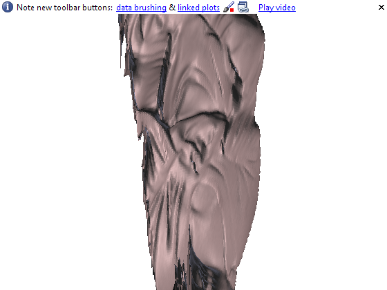
So, follows are some result images. The order is albedo, normal, normal arrow plot, depth, surface

And just a bunch of images of surfaces from different angles...

Implementation Details and discussion

Lighting Directions

To calculate the centroid of the chrome ball, I find x and y indices of non_zero values in the mask and average them.
Then, to get radius, I use the area calculate as the number of nonzero mask values.
The centers for the specular highlights on the chrome ball are done similarly.

Normals

Normals and albedo are both pretty basic implementations. Simply implement the algorithm. I used the weight function as in P2.

Depth

Issues

The primary difficulty that this reconstruction technique has is with shadows and specular(or very dark regions). A great example of this is the owl's eye.

Extension: Arbitrary light source

Not much to say about this, implement the algorithm and let it go. My results for this are significantly worse than those for the standard method.
Results from this method on the buddha dataset followed by that from the standard.

Extension: Example-based

So, I implemented the full algorithm for this. Then I went to run it on the fish dataset, let it run for 8 hours overnight... and it was about 10% down in the morning and I didn't have

another 60 or so hours to let it run. So, I am not sure how the results for this would turn out.

Files submitted

Results folder

Basically this folder contains this html report, and then all the image results.

Code folder

So there is a bit in here, most of it is simple utility functions.

IO stuff

write_data.m, write_image.m, read_data.m, read_image.m, read_normals.m, read_albedo.m, get_filename.m

These are all simple utility things. Some of the read functions do some very simple processing on the data.

Processing scripts

process.m, quiver_plot.m, surface_map.m, surface_images.m

These are basically just scripts to process a dataset and produce some output images. process.m is the leader.

The main stuff

get_lights.m, get_light_ex.m, get_centroid.m

get_lights is the main function to determine light directions. It uses the other two to do some of its work.

get_normals.m, get_albedo.m, get_depth.m

calculates normals, albedo, depth respectively. Implementation is discussed a bit above.

Extras

Arbitrary light sources

solve_arbitrary.m

Implementation of the algorithm for finding normals with arbitrary light sources.

Example-based

example_based.m

Implementation of the algorithm for finding normals from examples.

diffuse-specular separation

separate.m

Implementation of an algorithm to separate diffuse and specular components... doesn't really work.