Photometric Depth Reconstruction

Mikola Lysenko

Process

The objective of this project was to reconstruct a depth field from a series of photographs taken under controlled lighting conditions. The basic idea behind this process was to compute an approximation of the surface normals, which we then use to find a good approximation of the surface. We do this in four steps; first, we calibrate the camera by computing the lighting directions. Next, we find the normal map using least squares. Then, we solve for the color albedo using the normal data. Finally, we fit a surface using least squares again.

Camera Calibration

To perform calibration, we first gather a series of photographs of a chrome sphere taken under similar lighting conditions. From this, we determine the center of the sphere, $c$, its radius, $r$, and the location of the specular highlight in each image, $s_i$. To compute the light direction in each image, we use the fact that the normal for the sphere at the specular highlight is:

$$n_i = \frac{1}{r} \begin{pmatrix}s_{i,x} - c_{x} \ s_{i,y} - c_{y} \ \sqrt{r^2 - (s_i - c)^2} \end{pmatrix}$$

Assuming the camera is viewing the object head on, the viewing direction is then $v =\begin{pmatrix}0 & 0 & -1\end{pmatrix}$. From this, it is possible to solve for the lighting direction, $l_i$, using the standard reflection formula:

$$l_i = v - 2 (n_i \cdot v) n_i$$

Normal Reconstruction

The basic procedure for normal reconstruction follows from the project description. For each point in the image, we attempt to find a good normal by minimizing the following function at each pixel:

$$Q = \displaystyle\sum\limits_{i} (w_i I_i - w_i l_i g_i^T)^2$$

where $I_i$ is the intensity of the pixel in the $i^{th}$ image, $l_i$ is the light direction, $g_i = k_d n_i$ is the combined normal/albedo and $w_i$ is a weighting factor. For a weighting function, we chose to use the same function from the HDR project as suggested, giving:

$$w_i = 0.5 - \vert.5 - I_i\vert$$

which favors intensity values within the camera's dynamic range over specular/shadowed regions. The system of equations in the above is repeated for each color channel, giving a total of $3i$ constraints and $3$ unknowns. To reconstruct the normal, we solve the least squares problem using the conjugate gradient method as it is fewer lines of MATLAB code. This gives us a solution for $g_i$. To recover the normal directions, $n_i$, we simply unitize $g_i$.

Albedo Reconstruction

To find the albedo, we apply the formula described in the notes. For every pixel/color channel, we have:

$$k_d = \frac{ \displaystyle\sum\limits_{i} I_i l_i n_i^{T} } { \displaystyle\sum\limits_{i} (l_i n_i^T)^2 }$$

which can be solved directly using a loop over the image.

Surface Reconstruction

The final phase of the algorithm is surface reconstruction. To find the surface, we use the two orthogonality constraints as mentioned in the notes:

$$n_z z_{i+1,j} - n_z z_{i,j} = -n_x$$

$$n_z z_{i,j+1} - n_z z_{i,j} = -n_y$$

Along with the additional constraint that $z_{i,j} = 0$ for all points not in the image. To solve this large system, we use the preconditioned conjugate gradient method. On average, about 2000 iterations were necessary for convergence.

Software

The software for this project was written in MATLAB. All necessary files are included in this archive. To install the program, simply extract the files into a folder, then place the psmImages directory within the same folder. Because the images provided are in .tga format, you must have the tgatoppm and ppmtopcx utilities in your command line path and be using some form Unix. Once this is done, you may run the program to reconstruct a scene using the following MATLAB command:

reconstructObject('psmImages/objectName')

Where objectName is the directory containing the images of the object you want to reconstruct (eg. owl, horse, buddha). The program assumes a naming scheme the same as the sample files and requires that each sample is named something like object.1.tga and that there is a mask of the image labeled object.mask.tga.

Results

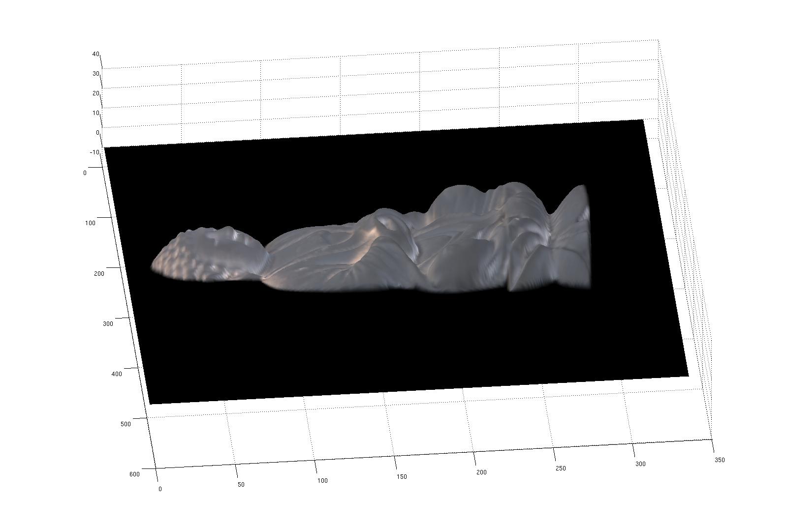
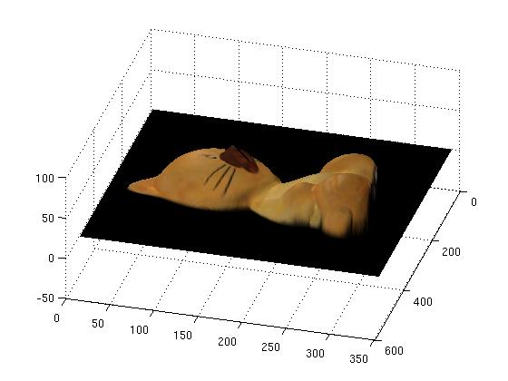
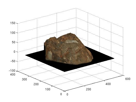
Overall, my implementation of this algorithm was quite successful, owing mostly to the nice test data kindly provided by the grader. In the following figure, we can see several reconstructed views of the buddha, horse, cat and rock:

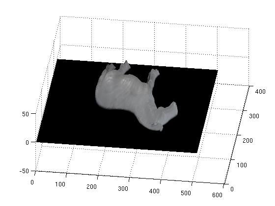
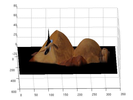
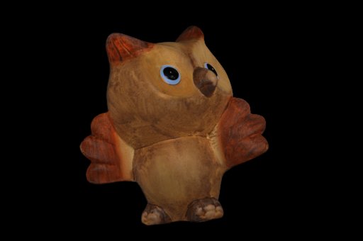
However, for the owl data set we ran into some problems as can be seen in the following reconstructed view. The spike in this picture is an unfortunate consequence of the high specularity on the owl's eye. This can be seen in the corresponding normal map, where there is a discontinuity.

Because of the fact that my previous project took so much time, I decided not to implement any enhancements for this particular exercise (other than the improved weighting.) However, the final product works and was completed on time, so there really isn't much to complain about.

The basic idea of computing a surface from its normals works pretty well. However, the method for determining the normals we used in this project is probably not the best. As mentioned in class, we could easily eliminate the requirement that we have a chrome sphere in the scene by estimating the lighting and normal direction simultaneously.

A major issue in this algorithm is that it doesn't work very well for specular objects. To get around this it might be possible to exploit the fact that specular reflection preserves polarization. Using this trick, we could estimate the degree to which the polarized light was rotated, giving the surface normal while allowing the specular components to be cancelled out.