Project 3: Photometric
Stereo
Yancan Huang, Shengqi Zhu,
Jiasi Song
Contents
4. Least
Square Surface Fitting
5. BONUS:
Estimating surface normals without using the chrome balls.
6. BONUS:
Weighted surface reconstruction
Bonus Points
We implemented two bonus points: estimating without chrome ball and weighted surface reconstruction. We also tried to reconstruct our own image, but the result is not good.
Collaboration:
Jiasi mainly implements calibration (step 1) and normal vector part (step 2), Shengqi mainly implements color albedo (step 3) and estimating without chrome ball (bonus 1), Yancan mainly implements surface fitting (step 4) and weighted surface reconstruction (bonus 2).
Input & Output:
To run the program, simply run basic.m
To change the input image, modify line2 in basic2_1.m:
inputfile = 'psmImages\buddhan.txt';
To run bonus point 1 (Estimating without chrome balls): run photometric.m
To run bonus point 2 (Weighted surface reconstruction): substitute “basic4” with “bonus4” in “basic.m” file, and rerun basic.m.
The program will automatically draw figures on the screen.
NOTE: Since matlab cannot read tga files, those files should be converted to other matlab-accepted files (such as bmp files) before running our programs.
Implementation Details
1. Calibration:
Code is in basic1_1.m and basic1_2.m.
A.In this part, the centre and radius of the chorme ball is calculated.
We use the way to calculate centroid to get the centre:
X0=sum ( x*grayValue(x,y))/sum(grayValue(x,y))
Y0=sum ( y*grayValue(x,y))/sum(grayValue(x,y))
The centre of the ball is (148.75, 254.25):
The radius of the ball is 118.2644
B. Calculate the centre of the brightest spot of 12 images of chrome balls:
Here we use the same way as calculate the centre of ball, but just count the pixels with gray value > 200, and get the brightest spots’ centers of 12 images as:
( 118.7593, 286.1258)
( 140.4816, 268.9597)
( 138.3136, 252.0241)
(121.6145, 248.3922)
(116.8895, 234.3231)
(113.6359, 247.3671)
(122.6177, 271.6766)
(122.3650, 260.4830)
(128.4637, 266.8056)
(128.6107, 259.6218)
(146.0096, 262.0192)
(126.7680, 245.6548)
C. Then, we use the results before to calculate the Lighting Direction of 12 images of chrome ball.
L=2(N.R)N-R ;
R=(0,0,1);
N=BrightestSpotCentre-BallCentre;
Below are the normalized lighting directions of 12 images:
( 0.2507, -0.2664, 0.9307)
( 0.0691, -0.1230, 0.9900)
( 0.0872, 0.0186, 0.9960)
( 0.2268, 0.0490, 0.9727)
( 0.2663, 0.1666, 0.9494)
( 0.2935, 0.0575, 0.9542)
( 0.2184, -0.1457, 0.9649)
( 0.2205, -0.0521, 0.9740)
( 0.1696, -0.1049, 0.9799)
( 0.1683, -0.0449, 0.9847)
( 0.0229, -0.0649, 0.9976)
( 0.1837, 0.0718, 0.9803)
2. Normals from Images
In
this part, we use the formula below to calculate the normal of each pixel of
the image:
![]()
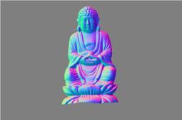
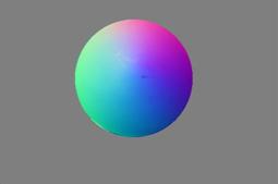
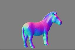
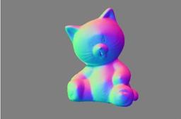
To
evaluate the performance of the algorithms, we produce a RGB image, with R,G,B
representing x, y, z respectively:
3. Solving for color albedo
Since we’ve already got the normal vector of each pixel, solving for color albedo becomes a simple calculation. For every pixel, we have

Here, the calculation is done in each channel separately. We have the following result for color albedo:
4. Least Square Surface Fitting
In this part, we aim to find the surface that has those normals calculated in part 2. As suggested in the Project Instructions, the principle here is: if the normals are perpendicular to the surface, then they will be perpendicular to any vector on the surface. We can construct vectors on the surface using the edges that will be formed by neighboring pixels in the height map.
Consider a pixel (I, j) and its neighbor to the right, they will have an edge with direction:
![]() .
.
Since this vector is perpendicular to the normal n, so its dot product with n will be zero:
![]() , i.e.,
, i.e., ![]() .
.
Similarly, in the vertical direction, we have:
![]() .
.
We can construct in similar way all
constraints for all the pixels which have neighbors, and we can rewrite this
linear system as matrix equation: ![]() , in which the number of equations are about twice of number
of variables.
, in which the number of equations are about twice of number
of variables.
In practice, the size of M is more than 10000*10000 (take the ‘cat’ images as example, the size of M is about 60000*30000) and most entries are 0, so we use sparse matrix to represent this large matrix.
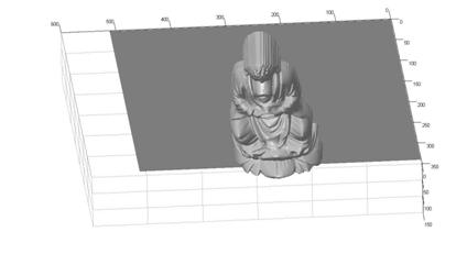
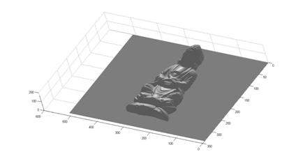
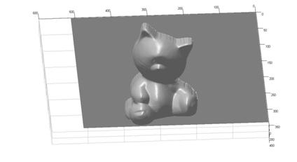
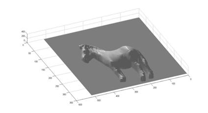
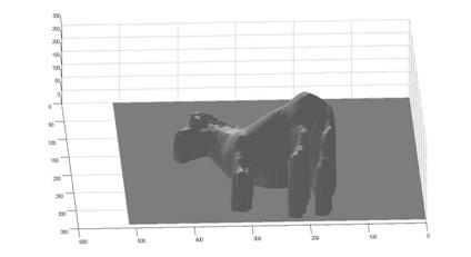
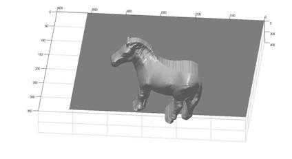
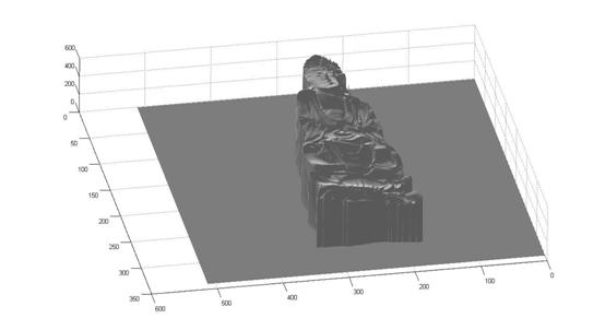
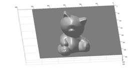
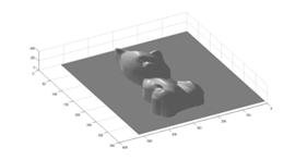
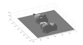
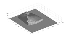
Finally, we list here different views of the reconstructed surface without albedos:
² buddha
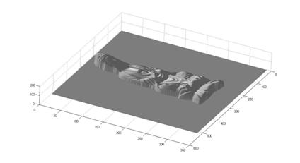
² cat

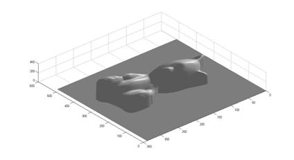
² horse
5. BONUS: Estimating surface normals without using the chrome balls.
This part was referred to Hayakawa’s paper “Photometric stereo under a light source with arbitrary motion”. The main idea here is to use SVD to estimate both the light direction and surface normal simultaneously. Here, suppose we have a series of pictures with p pixels through f frames. We first pile all the pixels up to form a matrix:

Here, ![]() , where R is the surface reflectance matrix, N is the surface
normal matrix, M is the light-source direction matrix and T is the light-source
intensity matrix.
, where R is the surface reflectance matrix, N is the surface
normal matrix, M is the light-source direction matrix and T is the light-source
intensity matrix.
One characteristic of these four matrices
is that R and N only depend on pixel p while M and T only depend on frame
f. This property made it possible
for us to estimate RN and MT simultaneously if we have a series of images. More specifically, we know that the rank
of RN is 3 and rank of MT is 3 as well.
Therefore, by using SVD, we can decompose I into 2 different
matrices. If we do SVD, we get ![]() . Since we have
noises in the images,
. Since we have
noises in the images, ![]() is very likely to
be a matrix with rank more than three.
We can choose the largest three components in
is very likely to
be a matrix with rank more than three.
We can choose the largest three components in ![]() , and make other components to be zero. In such way we get a decomposition of I
as
, and make other components to be zero. In such way we get a decomposition of I
as
![]()
![]()
However, there is still one ambiguity here. For any invertible 3x3 matrix A, we
could also have ![]() and
and ![]() . We must do some
assumptions here in order to resolve this ambiguity. Here, we assume that the relative value
of the light-source intensity is constant.
Then we have
. We must do some
assumptions here in order to resolve this ambiguity. Here, we assume that the relative value
of the light-source intensity is constant.
Then we have
![]()
Here, we let ![]() , it has 6 degrees of freedom (since B is a symmetric
matrix). We can solve for B using
any standard over-determined linear equations approach, such as Least Square
Estimations. As long as we get B,
we could do another SVD decomposition
, it has 6 degrees of freedom (since B is a symmetric
matrix). We can solve for B using
any standard over-determined linear equations approach, such as Least Square
Estimations. As long as we get B,
we could do another SVD decomposition
![]()
Therefore, we can easily get A from B, and hence get S and L matrix.
Here, we show some
RGB encoded normal vector results:
The first one is
the buddha sample. However, this
time we did not use the chrome ball information.
The 3D surface is worse than using chrome ball. We think there might be 2 reasons to account for this situation. First, we are using less information to estimate the same object; second, the assumptions of constant light-source intensity might not hold.
The second one is a box, which was photographed by ourselves, using the following series of images:
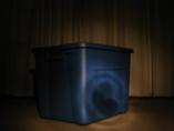
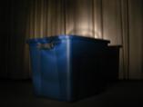
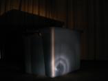

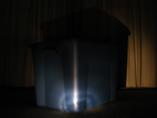
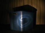
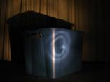
The generated RGB-encoded normal vector image is shown below. This algorithm clearly separated different surface and showed it with different colors. We also see some circle noises in this image. It is due to the high reflective effect when using a torch. We also noticed that the original bin is too dark, making it difficult to reconstruct the whole object.
6. BONUS: Weighted surface reconstruction
As suggested in Project Instructions, we modify the objective function for surface reconstruction by weighing each edge constraint with some measure of confidence according to the brightness of the pixel. In another word, we want the constraints for dark pixels where the normal estimate is bad to be weighted less heavily than bright pixels where the estimate is good.
In practice, we assign each equation with some weight, for which we choose the ratio of the current pixel’s intensity vs. the average intensity.
Finally, we list here multiple views of the basic and weighted reconstruction results for comparison:
² cat: Left two pictures are from basic approach, right two pictures are from weighted reconstruction method.

² box: Left picture is from basic approach, right picture is from weighted reconstruction method.
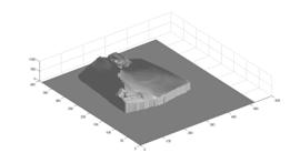
From comparison, we can that the weighted version of surface reconstruction approach performs much better than the basic method. For example, the details of the cat eye are much clearer in the right two pictures which are calculated with weighted reconstruction approach; and the box surface are much smoother in the right ‘box’ picture which is calculated with weighted reconstruction method.