Computer Vision Project Report 3

Photometric Stereo

Yupu Zhang

yupu at cs.wisc.edu

Goal

To implement a system that constructs a 3D height field image from a series of 2D images of a diffuse object under different point light sources

Steps

1  Calibration

There is only one step remaining left for us: calculate lighting directions using the “chrome ball” method. I follow the hints mentioned in the project page to complete this step. Note that I apply an intensity-weighted method to calculate the centroids of the ball mask, as well as those of the highlight pixels. Here is how to do it in MATLAB and it’s pretty simple.

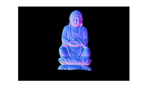
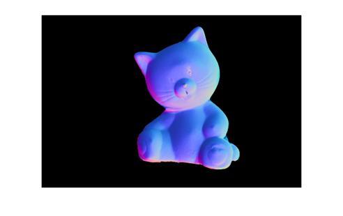
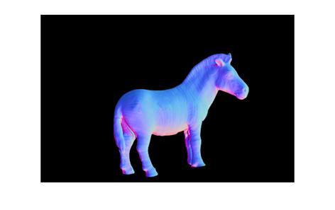
2  Normals from Images

Basically, it’s a linear least squares problem. Suppose that I is the pixel intensity, kd is the albedo, n is the normal vector and L is the lighting direction, and let g = kd*n, I could get the object function (after weighting the solution by I). The normalized g is n.

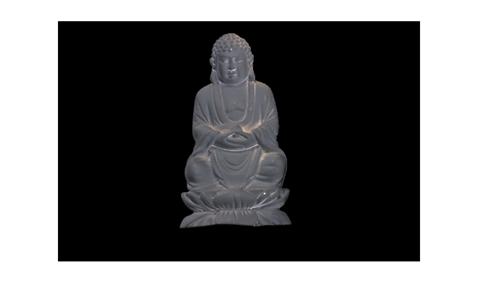
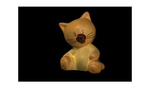
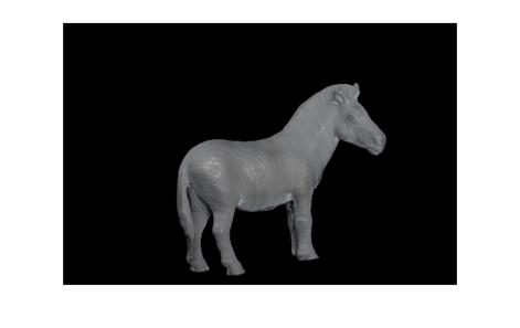
3  Solving for color albedo

It’s also a linear least squares problem. For one channel, the object function is:

I solve it by differentiating it with respect to kd and setting it to zero.

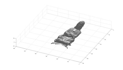
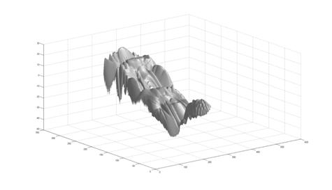
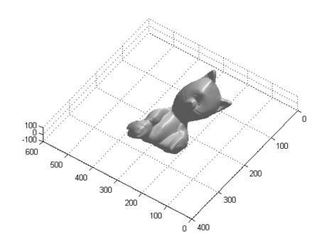
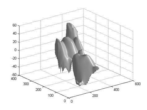
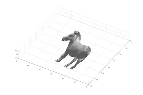
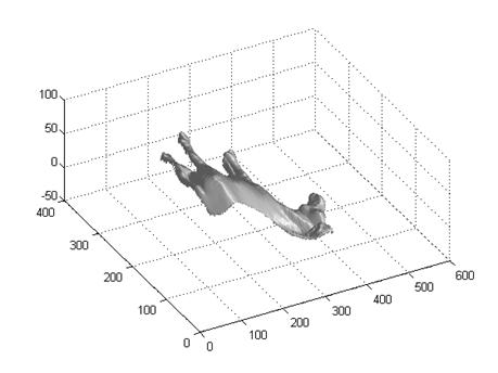
4  Finding the surface

In this step, I apply the method suggested in the project page. By adding two constraints to each pixel of the image, I can pose this problem as another least squares problem: Az = b. Since A is a huge matrix, I use a sparse matrix to represent A in MATLAB and then solve the linear system by using ‘A\b’.

How to Run

My program is implemented in MATLAB. The function header is below:

function stereo(imgsetname)

where ‘imgsetname’ is one of the following strings: ’buddha’, ’cat’, ’chrome ’, ’gray’, ’horse’, ’owl’, ’rock’.

All images are converted into PNG files manually and stored in the same dir structure as the original image set package). The three required plots will show up in the end.

Results full size plots can be found here

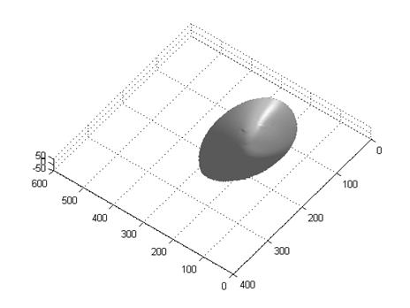
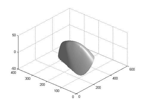
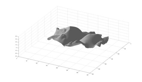
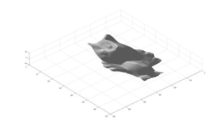
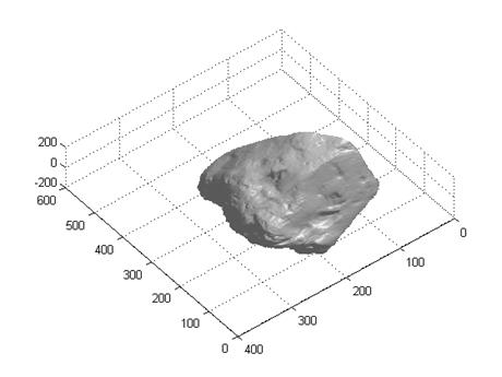
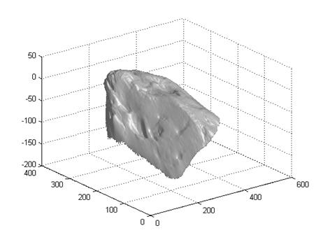
In the surface plot, in order to make it nice (easy to see the shape of the objects we are interested in), I set the height of the pixels that are outside of the mask to NaN (null in MATLAB).

1  Buddha

2  Cat

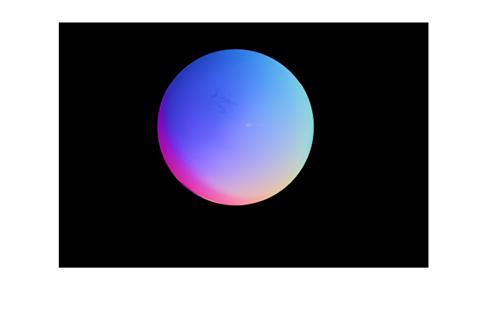
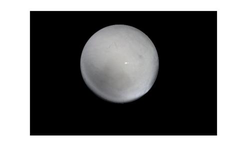
3  Gray

4  Horse

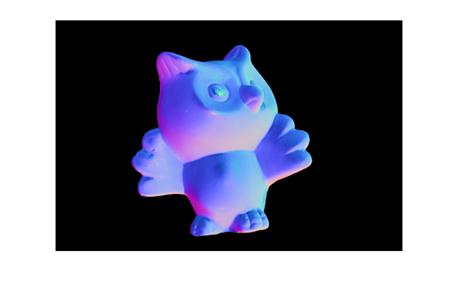
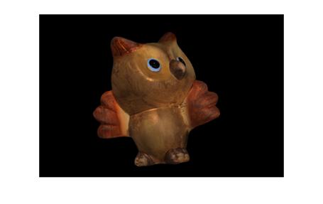
5  Owl

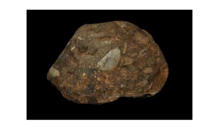
6 Rock

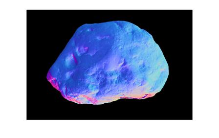
Discussion

The result looks good but I find two problems here. One is that the 3D shape of the gray ball is not right. I guess it’s due to the error of the method itself. The reason why other objects look good might be that they are not so regular as the gray ball that we just can’t tell the small differences between the original shape and the reconstructed shape. The other one is the eye of the owl, which appears to be a spike in the surface plot. It’s because the area of the eye is too dark (saturated). I think a good weighting function or smooth function might solve this problem.