I. Running Our Program
Our program is written in Matlab, and thus, must be run inside Matlab (no standalone executable). To run our program, simply navigate to our project folder and type the following:
panoramaker( nameOfDirectoryOfImages, focalLength );
where nameOfDirectoryOfImages is a directory of input images to use for the panorama algorithm. DO NOT include a trailing slash on the directory name. You may optionally leave off the focalLength parameter, in which case, it will default to 661, the focal length for all of our images.
Note: The algorithm assumes that the alphabetical order of the images corresponds to the images panning over the underlying scene right-to-left.
Note: If running on on Linux, you may need to give the sift executable permission to run. (It is something used by the David Lowe sift algorithm). To do so, just do the following:
cd to our project’s root directory
chmod +x sift
Performance
Given a set of 18 images, the program takes about 40 minutes
to go from a set of raw images to a fully-stitched panorama.
As a performance shortcut, our program can cache cylindrical projection images
so that they only have to be computed once.
II. Implementation Details
Our program is composed of a 5-stage pipeline:
- Cylindrical Projections
- Alignment Computations
- Drift Correction
- Stitching and Blending
- Cropping
We describe each of these stage in turn:
Cylindrical Projections
We perform our cylindrical projections via inverse mapping. From each destination (x,y), we compute the source (x,y) coordinates from the following formulas:
sourceXs(y,x) = focalLength * tan( (x - imgWidth / 2 )/s) + imgWidth / 2;
sourceYs(y,x) = focalLength * (y - imgHeight /2 ) / s * sec( (x - imgWidth / 2) / s ) + imgHeight / 2;
Each cylindrical projection is then saved in a temporary cylindrical directory as a png image. To speed up testing, our program supports the caching of these cylindrical projections, and if it notices that they already exist, will skip this step in the pipeline entirely.
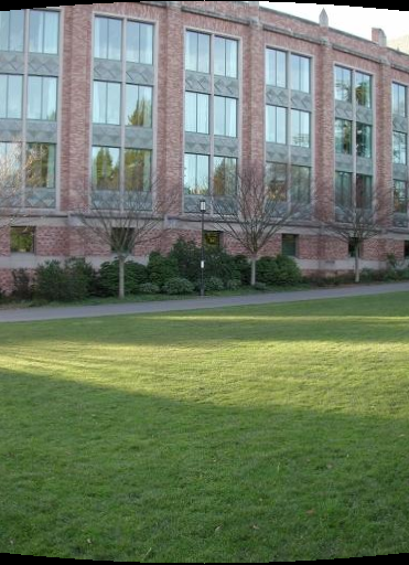
An example cylindrically-projected image
Alignment Computations
Armed with our cylindrical projections, we then compute the translation needed to go between each pair of consecutive images. We do this via the following procedure:
For each pair of images:
- Extract features and descriptors of each image using the David Lowe Sift program.
- Get a mapping of point correspondences using a match procedure adapted from the David Lowe files.
- Perform RANSAC for a number of iterations:
- Select 1 random point correspondence.
- Compute the homography (translations x,y) needed to transform one image into another.
- Transform that image using those translations
- Re-apply the matching procedure to identify the matching points between the transformed image and the original second image.
- Count number of inliers, which we define to be point correspondences with locations falling within 2 pixels of each other.
- If a new maximum number of inliers
- Compute an additional homography using all of the inliers.
- Add this additional homography into our original homography and store it as our new “best” homography
- Output our best homography
Some Notes:
Only one point correspondence is needed at each iteration, since two equations is necessary to solve for the two unknowns: translation in x and y.
We found that this stage performs decently with just 2 iterations, but we’ve increased it to 10+ iterations to produce results with a higher confidence level.
Drift Correction
To correct and prevent the buildup of y translation drift,
we normalize all y translations such that they all sum to 0.
We do this prior to doing stitching and blending.
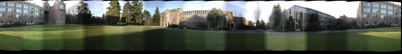
 Above is an initial panorama we created, prior to our implmenting
of drift correction.
Above is an initial panorama we created, prior to our implmenting
of drift correction.
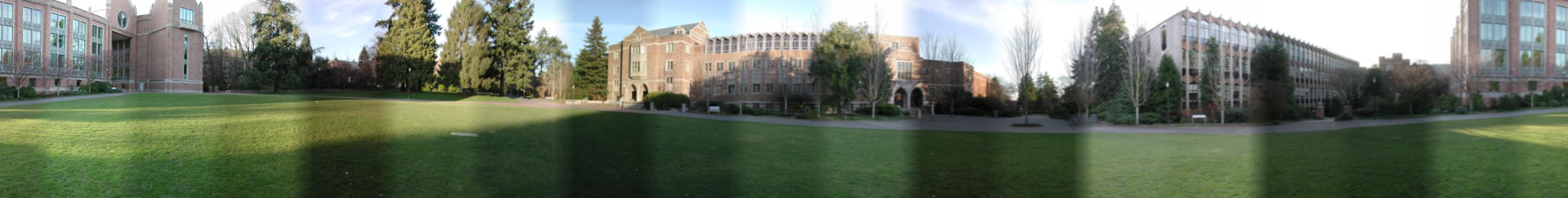
 Above is our panorama with drift correction, but before cropping.
Stitching and Blending
Our stitching procedure works by iteratively building up the
image right-to-left. At each iteration, we take a new left image
and add it into the right image.
- Calculate the new size of our combined image
- Create two images of the new size. Call these L and R.
- Copy the left image into the left side of L and the right image into the right side of R.
- Blend the two images into a final combined image. We have implemented both feather blend and pyramid blend.
Cropping
Our original implementation of final image cropping calculated the maximum image offset in the vertical axis based on the translations reported by the image alignment step. This would allow us to perfectly crop off the unwanted black regions created from the cylindrical reprojections and translations. However, for reasons unknown, these numbers did not translate well to the actual required cropping amount. To fix this, a linear search was done to find the most black pixels in a row from top and bottom to determine the amount to crop.
 Above is our final panorama of the testing images, with cropping
and drift correction.
Above is our final panorama of the testing images, with cropping
and drift correction.
III. Extensions
We implemented a number of extensions, and describe each in turn:
Pyramid Blending
Our pyramid blending module works by taking a left image and right image as inputs. From there, it follows these stages:
-
Create a gaussian pyramid of both the left and right images
-
Use the Gaussian pyramids to create laplacian pyramids of both the images
-
Identify a boundary line to use as the boundary of where the left image ends and the right image begins.
-
Create a combined laplacian pyramid by copying the left and right laplacian pyramids into their respective parts of the combined pyramid. The pixels directly on the dividing line are set to the average of the left and right image pixels of that location. Repeat this for every level of the combined pyramid.
-
Collapse the laplacian pyramid to acquire the final image.
Our pyramid uses 4 levels. We tweaked a number of parameters with it, including the number of levels and the gaussian filter, but disappointingly, we found that it didn’t work as well as the feather blending.
Exposure Correction
Our exposure correction takes in two images and attempts to
find the average intensity for similar colors. It does this via the following steps:
- Bin colors based on their RGB vector direction
- Calculate the average intensity of each bin
- Calculate the required shift of each bin’s distribution the yields the greatest overlap.
- Apply the shift to each pixel, weighting the correct bin’s shift value according the pixels proximity to the paired image.
The method did not produce very desirable results. If the bins were too large, too many colors were affected, producing blotchy areas. If the bins were too small, there were not enough colors in each bin to usable data. This method works great if you want to take two images and make them look like sponge paintings.
IV. Final Results
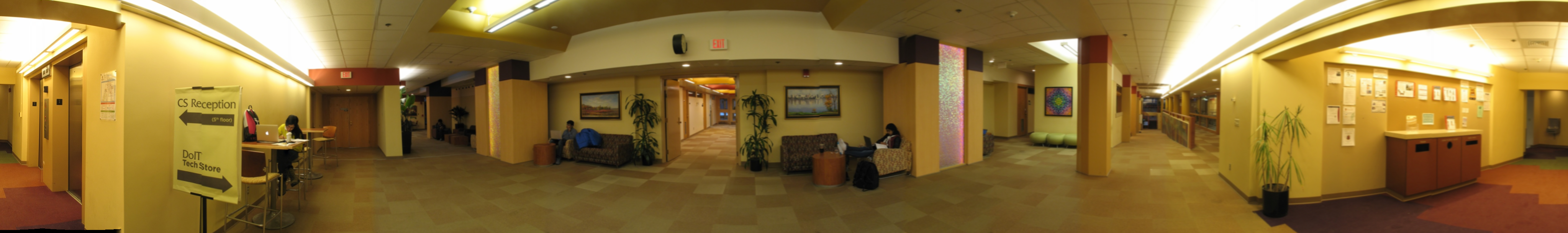
Below are our results of the entire process. Click on any
image for a zoomed-in view, or click on the link below each for
the panorama-viewer. Each of these was created using 5 RANSAC
iterations and feather blending with a window size of 50.
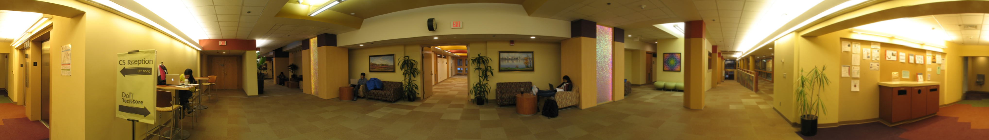
View in panoramic viewer.
A panoramic view of the CS lobby.
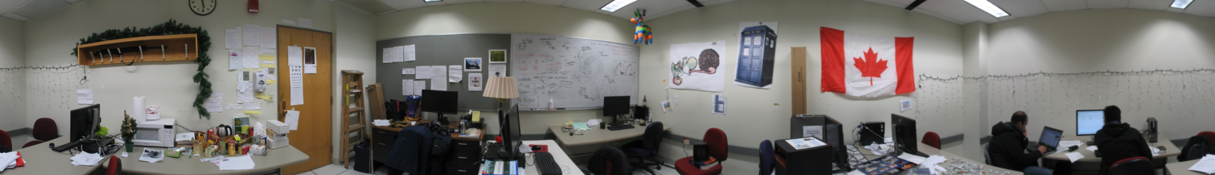
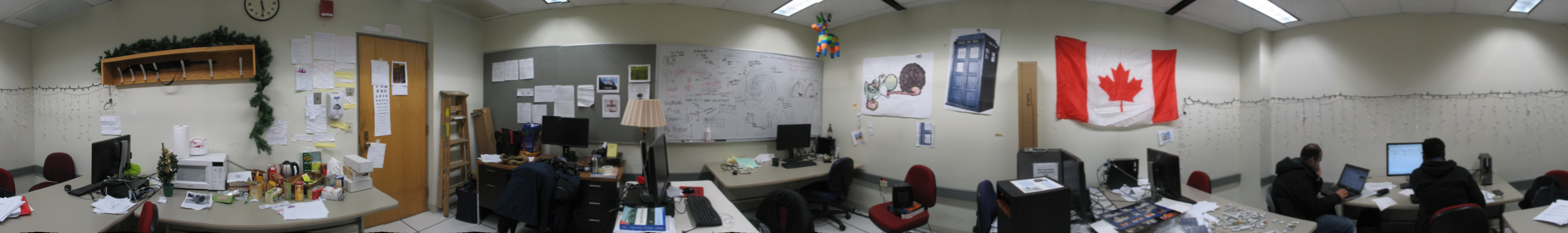
View in panoramic viewer.
Stephen's office, 1351 CS, "Terminal Room B".
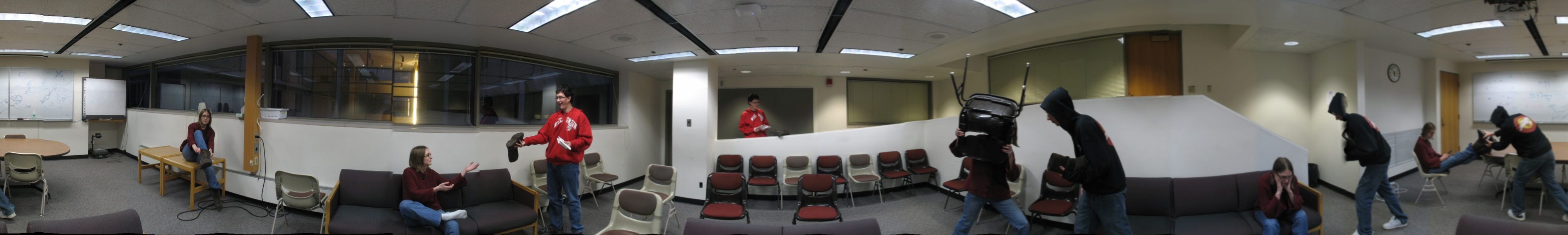
View in panoramic viewer.
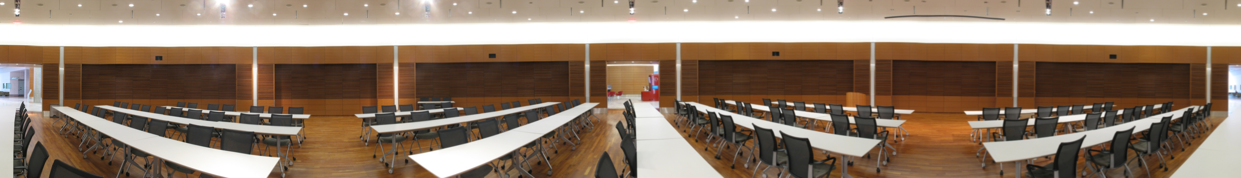
The provided Testing Images.
View in panoramic viewer.
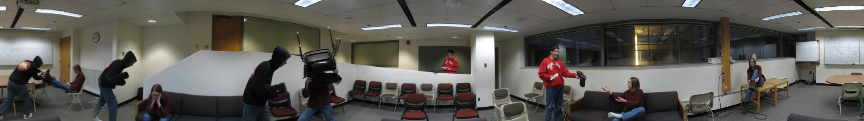
A fun action panorama of a thief stealing a boot.
View in panoramic viewer.
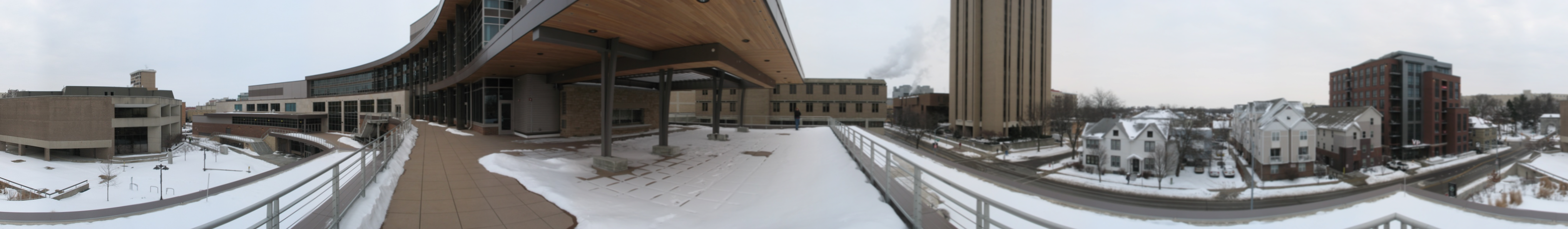
The back balcony of Union South looking upon Dayton St.
View in panoramic viewer.
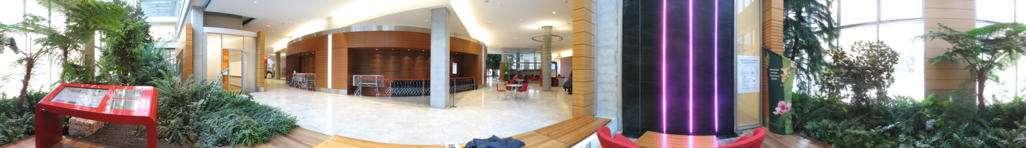
By the Fibonacci chimes area in the WID lobby.
Pyramid Blending Results
We also created a few panoramas with pyramid blending, but found
that it did not work as well as feather blending. In particular, we
found that it left some very noticeable seams and misalignments.