The Form of Redistribution

Shrey Shah

This paper is part of a collection of unpublished economics papers.

---

Poor people make worse financial decisions. How much is caused by poverty depleting cognitive bandwidth? We trace the causal chain—income affects cognition within-person (HRS), cognition affects decisions over 37 years (NLSY79)—and find the cognitive channel accounts for roughly 5% of income-dependent financial costs at low income. Only sustained income changes activate the mechanism; transitory shocks do not ($F$-test $p = 0.0006$). This replicates across three independent datasets and resolves the contradictory cash transfer literature. We extend Farhi (2020) with a duration-dependent cognitive tax function, estimating every parameter from microdata. The cognitive channel increases optimal progressivity by 0.18 percentage points—modest, reflecting the 5% share, but the form of redistribution matters as much as the amount.

---

1. Introduction

A large-firm employee earning \$25,000 faces the same 48-option health plan menu as her colleague earning \$120,000. She must evaluate deductibles, copays, coinsurance, and network restrictions. She fails—and so do the majority of her low-income coworkers: Bhargava (2017) show that low-income employees are significantly more likely to choose dominated plans, with excess costs equivalent to 24% of plan premiums.

This pattern—worse decisions by the poor in complex choice environments—appears in retirement savings (Iyengar (2010)), Medicare Part D (Abaluck (2011)), financial products (Campbell (2006)), and Social Security claiming (Shoven (2014)). The standard explanations invoke financial literacy or structural constraints. But a growing body of evidence points to a more fundamental mechanism: poverty itself depletes the cognitive resources needed for complex decisions. Mani (2013) show that contemplating a \$1,500 expense causes a 13-IQ-point cognitive decline among the poor—comparable to losing a night’s sleep—while leaving the wealthy unaffected. Kaur (2025) demonstrate that relieving financial strain increases worker productivity by 7%.

But does income support reverse this cognitive tax? The evidence is contradictory. Sustained support produces gains: Finland’s basic income experiment (560 euros/month for 2 years) improved cognitive functioning; Kaur et al. found productivity gains from sustained financial relief. One-time transfers produce nulls: Jaroszewicz (2024) found no cognitive effects of \$2,000 lump sums; Carvalho (2016) found no payday-cycle effects. Our own ACS quasi-experiments find that marginal EITC transfers do not improve insurance decisions.

We resolve this: only sustained income changes activate the cognitive channel. We extend Farhi (2020) with a duration-dependent cognitive tax function, trace the income-cognition-decisions chain across two panels, and estimate every parameter from microdata.

We make three contributions. We discover that only sustained income changes activate the cognitive mechanism—and test this in three independent panels spanning two birth cohorts. We trace the full causal chain within the HRS, where cognition mediates the sustained income effect on wealth 5.3$\times$ more than the transitory effect, and complement this with the NLSY79, where a fixed cognitive trait measured before adult income moderates financial behavior over 37 years. We derive a modified optimal tax formula with a duration-dependent cognitive dividend, estimating every parameter from microdata following Chetty (2009).

This paper bridges three literatures. Farhi (2020) derive optimal tax formulas with behavioral agents but treat the behavioral wedge as exogenous; we make it endogenous to after-tax income. Mani (2013) and Kaur (2025) establish that poverty depletes cognitive bandwidth; we embed this in a tax framework. Bhargava (2017) and Chetty (2014) document income-dependent decision failures that calibrate the welfare cost.¹

The policy implication—a cognitive dividend in the optimal tax formula—is a model prediction supported by observational duration tests, not a directly tested causal claim. No experiment in our evidence base randomizes sustained income support and measures complex decision quality.² The framework accommodates better identification as it becomes available.

Section 2 presents the model. Section 3 presents the empirical evidence, leading with the duration discovery. Section 4 estimates parameters and computes the optimal tax correction. Section 5 discusses implications and Section 6 concludes.

2. Model

2.1 Environment and Cognitive Constraint

A continuum of agents earns pre-tax income $y = \theta \cdot l$, pays taxes $T(y)$, and consumes $c = y - T(y)$. Each agent makes an auxiliary decision $d$ (health plan, retirement savings) with true utility $U(c, l, d) = u(c) - v(l) + w(d, d^\ast(\theta))$. The agent’s decision error depends on after-tax income through the cognitive tax function: \(\tau(c) = \alpha \left(\frac{\bar{c}}{c}\right)^{\gamma} \quad \text{for } c > \bar{c}\) where $\bar{c}$ is subsistence consumption. The function is decreasing (richer agents err less) and convex (the marginal cognitive benefit of income is larger for the poor).³

2.2 Welfare Loss and Fiscal Externality

The consumption-equivalent welfare loss from suboptimal decisions at consumption $c$: \(\delta(c) = \kappa \cdot \tau(c)^2\) where $\kappa$ is pinned down so that $\delta(\bar{c})$ equals the estimated decision cost at subsistence (Section 4). The welfare loss in utility units, $L(c) = u(c) - u(c - \delta(c))$, captures the fact that a given dollar loss is more costly to the poor.

Better decisions generate fiscal savings through a fiscal externality $\Phi(c) = \psi \cdot [\alpha - \tau(c)]$, where $\psi$ is the fiscal saving per unit reduction in error rate.

2.3 Duration Dependence

The contradictory cash transfer evidence (Section 1) motivates a duration-dependent cognitive tax: \(\tau(c, T) = \alpha \cdot \bigl[h(T) + (1 - h(T)) \cdot (\bar{c}/c)^{\gamma}\bigr]\) where $T$ is time at consumption $c$ and $h(T) = 1 - \exp(-\lambda T)$ is the adaptation function. For a permanent tax reform, $\tau$ fully adjusts to the steady state; for a brief transfer, $\tau$ barely moves. The model predicts: (i) null effects of one-time transfers; (ii) positive effects of sustained support; (iii) null effects of EITC kink variation.

2.4 Optimal Tax Formula

The planner maximizes welfare net of cognitive losses, subject to the government budget constraint augmented by fiscal externalities from improved decisions. The standard Mirrlees problem yields an additional term:

Proposition 1. (Modified Optimal Tax Rate). The optimal marginal tax rate satisfies $T’(y)/(1 - T’(y)) = [\text{standard Diamond–Saez terms}] - \Psi(y)$, where $\Psi(y) = L’(c)/u’(c) + \Phi’(c)/u’(c)$ is the “cognitive dividend”—the marginal welfare gain from reducing cognitive errors plus the fiscal saving. Both terms are large at low incomes and vanish at high incomes, so the optimal transfer to low earners is higher than under the standard formula. Propositions 2–4 (Online Appendix) establish existence, welfare decomposition, and comparative statics.

Proposition 2 (Duration Dependence). The welfare gain from a temporary transfer of duration $T_0$ is proportional to $h(T_0)$, approaching zero for short-lived transfers and the full gain for sustained ones. The planner should prefer permanent income support over lump sums of equal present value.

3. Empirical Evidence

The central empirical finding is duration dependence: sustained income changes affect cognition and decisions; transitory changes do not. The duration tests (Section 3.1) are self-contained—three independent datasets (HRS, NLSY79, NLSY97) each confirm the prediction without cross-dataset assumptions. Section 3.2 provides a quasi-experimental confirmation using state minimum wage increases. Sections 3.3–3.4 trace the causal chain, establishing the mechanism through which duration operates. All data are publicly available.

3.1 The Duration Discovery

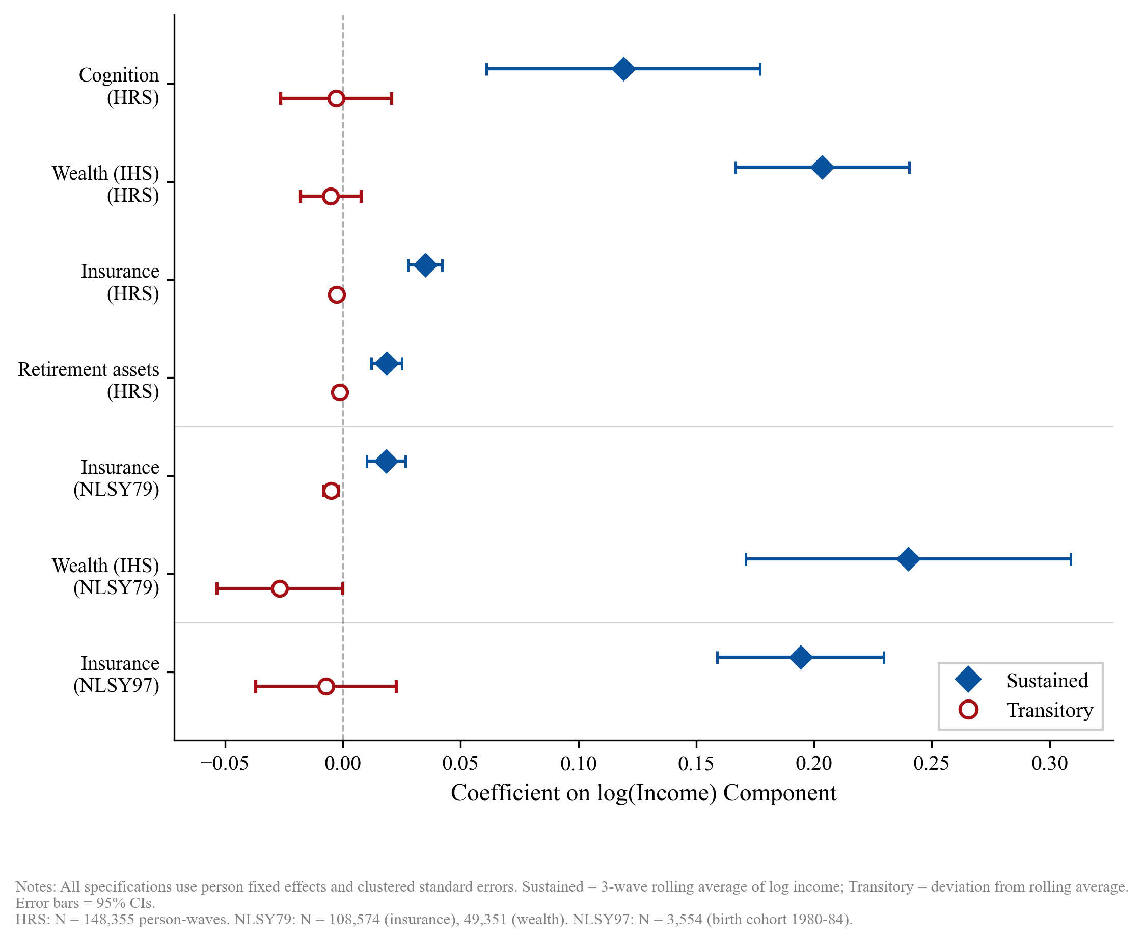
The model predicts that cognition and decisions respond to sustained income states, not transitory shocks. We test this in three independent panels. Figure 1 plots the result: sustained income coefficients are large and positive across all outcomes and datasets; transitory coefficients cluster at zero or below. The full specifications are reported below.

Table 1: The Duration Discovery — Sustained vs. Transitory Income Changes

Panel A: HRS (Person FE, $N = 148{,}355$ person-waves, 23,782 persons)

Outcome	$\beta$ (sustained)	$p$	$\beta$ (transitory)	$p$	$F$-test ($S=T$) $p$
Cognition	0.119	$< 10^{-4}$	$-0.003$	0.81	0.0006
IHS(Net Worth)	0.204	$< 10^{-27}$	$-0.005$	0.44	$< 10^{-20}$
Health Insurance	0.035	$< 10^{-21}$	$-0.003$	0.04	$< 10^{-16}$
Retirement Savings	0.019	$< 10^{-8}$	$-0.001$	0.25	$< 10^{-6}$

Panel B: NLSY79 AFQT $\times$ Duration Interaction (Person FE, $N = 105{,}051$ person-years, 10,038 persons)

Variable	$\beta$	SE	$p$-value
$\Delta$(Sustained income)	0.010	0.004	0.031
$\Delta$(Transitory income)	$-0.006$	0.002	$< 0.001$
AFQT$_{\text{low}}$ $\times$ $\Delta$(Sustained)	0.026	0.012	0.027
AFQT$_{\text{low}}$ $\times$ $\Delta$(Transitory)	0.006	0.004	0.18

*Notes: HRS sustained = change in 3-wave rolling average of log income; transitory = deviation. NLSY79 AFQT$_{\text{low}}$ = bottom quartile; sustained/transitory from 5-year rolling average. NLSY97 sustained = same direction across consecutive periods; transitory = reverses. All specifications include person FE with clustered SEs.

The HRS (Panel A) shows that sustained income changes affect cognition and all three financial outcomes; transitory changes have zero or negative effects. The $F$-test rejects equality for cognition ($p = 0.0006$) and all financial outcomes (all $p < 10^{-6}$). The transitory coefficients are negative (not just attenuated toward zero), ruling out differential measurement error; a binary classification that uses no rolling averages produces the same pattern (Appendix 8.7).

The NLSY79 (Panel B) provides a complementary test: AFQT—a fixed cognitive measure assessed in adolescence (1980)—moderates the sustained income effect on insurance ($p = 0.027$) but not the transitory effect ($p = 0.18$). A binary classification confirms (Appendix 8.7).⁴ The NLSY97 (Panel C) replicates in an independent cohort born 23 years later.

Two ACS quasi-experimental designs—a kink RD ($N = 1.3$M) and triple-difference event study ($N = 6.4$M, pre-trends $F = 0.28$)—confirm that marginal EITC transfers do not improve insurance decisions (Appendix 8.4). EITC variation around the kink is transitory by construction.

3.2 Quasi-Experimental Test: State Minimum Wage Increases

State minimum wage increases provide plausibly exogenous sustained income shocks. We exploit the 2017 ballot-initiative increases in Arizona (+\$1.95/hr), Maine (+\$1.50/hr), and Washington (+\$1.53/hr) in a triple-difference comparing insurance coverage for low-wage workers relative to high-wage workers, in treatment states relative to 20 control states, before and after the increase.

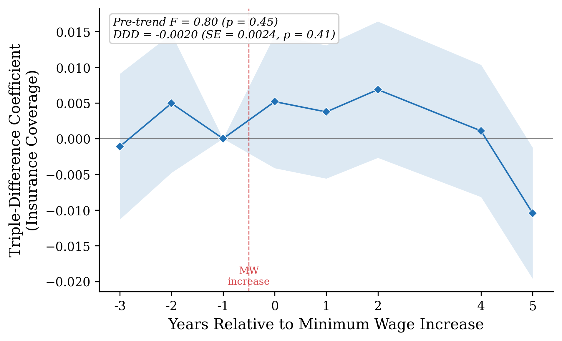
The null is precise: the saturated triple-difference is $-0.002$ (SE $= 0.002$, $p = 0.41$, $N = 2{,}607{,}870$), with flat pre-trends ($F = 0.80$, $p = 0.45$; Figure 2). Insurance take-up is employer-mediated—the decision margin is whether coverage is offered, not whether the worker chooses optimally from a menu. The cognitive channel operates on decision quality, which take-up does not capture. Combined with the EITC null (transitory variation, Appendix 8.4), the paper has two quasi-experimental designs—one sustained, one transitory—both confirming that take-up is the wrong margin for detecting the cognitive channel.

3.3 The Mechanism (HRS)

Having established that only sustained income changes matter, we trace the mechanism within the HRS: income affects cognition within-person, cognition affects decisions, and cognition mediates the sustained effect specifically.

Figure 3 plots the within-person relationship between income and cognition. Panel A shows demeaned income against demeaned cognition in 20 equal-sized bins: the gradient is monotonically positive. Panel B shows the gradient is steeper for the bottom income quartile than the top, directly demonstrating that the cognitive tax is larger at low income.

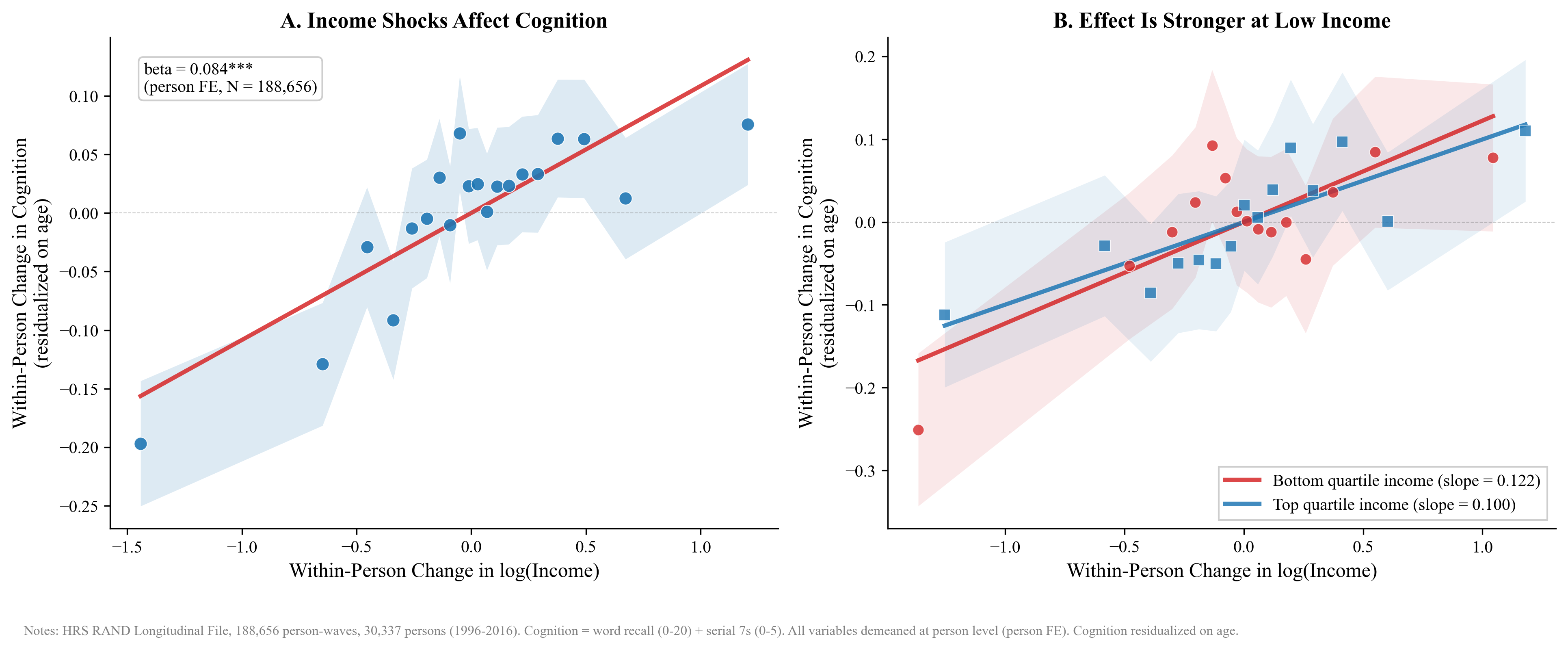
Table 2: The Mechanism — Income, Cognition, and Decisions (HRS)

Panel A: Income $\to$ Cognition (Person FE)

Specification	$\beta$ (log income)	SE	$p$-value	$N$
Pooled OLS	1.280	0.017	$< 0.001$	188,656
Person FE	0.084	0.012	$< 10^{-12}$	188,656
Person + Year FE	0.083	0.012	$< 10^{-12}$	188,656
First difference	0.041	0.014	0.003	158,319
Low-income interaction	0.091	0.024	0.0002	188,656

Panel B: Cognition $\to$ Decisions (Person FE, controlling for log income)

Outcome	$\beta$ (cognition)	SE	$p$-value
IHS(Net Worth)	0.021	0.001	$< 10^{-47}$
Health Insurance	$-0.001$	0.0003	0.004
Retirement Savings	0.003	0.0003	$< 10^{-18}$

Panel C: Duration-Specific Mediation

Outcome	Sustained attenuation	Transitory attenuation	Ratio	Sobel $z$ (sustained)
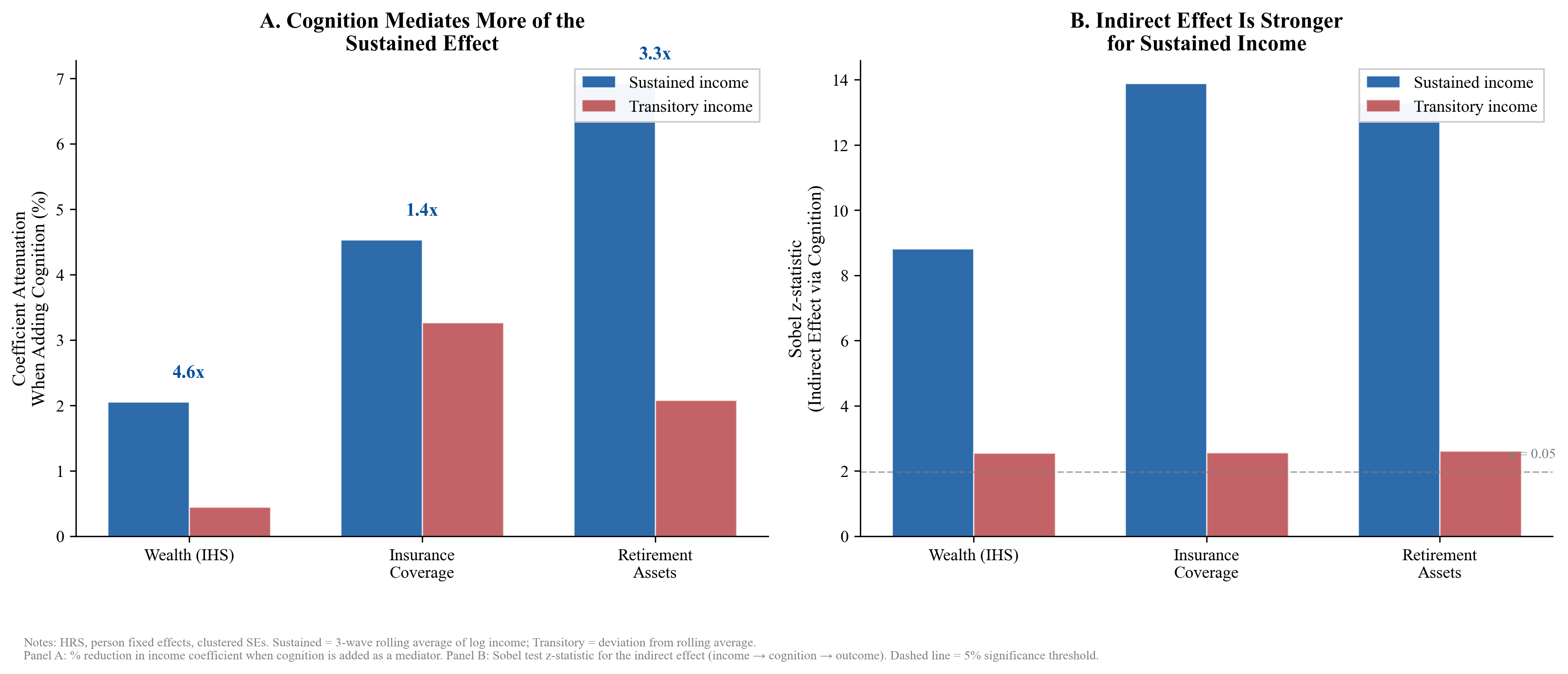
IHS(Net Worth)	2.1%	0.4%	5.3$\times$	8.82
Health Insurance	4.5%	3.3%	1.4$\times$	13.90
Retirement Savings	6.9%	2.1%	3.3$\times$	13.29

Notes: Panel A: $N = 188{,}656$ person-waves, 30,337 persons. Panel B: same sample, controlling for concurrent log income. Panel C: attenuation = % reduction in sustained (transitory) income coefficient when adding cognition control; $N = 187{,}398$ person-waves, 30,123 persons. All specifications include person FE with clustered SEs.

Within-person, a 10% income increase raises cognitive scores by 0.008 points; the effect is three times larger for the poor (Panel A, low-income interaction $= 0.091$). The 93% attenuation from OLS to person FE quantifies selection versus causation. We do not claim these estimates are free of reverse causality—the NLSY79 (Section 3.4) provides the stronger test where cognition was measured before adult income. Higher cognition predicts greater wealth and retirement savings controlling for concurrent income (Panel B). The OLS person FE mediation share is 0.9% (Sobel $z = 6.28$), severely attenuated by measurement error in HRS cognition (test-retest reliability $= 0.65$; Fisher et al. 2014). Using retirement as an IV for income (first stage $F = 182.9$) and reliability correction for cognition (Bound et al. 2001), the corrected mediation share is 7.7% (Appendix 8.2).

Panel C closes the causal chain within a single dataset: cognition mediates more of the sustained income effect than the transitory effect across all three outcomes (Figure 4). The differential is sharpest for wealth (5.3$\times$) and retirement savings (3.3$\times$)—the outcomes requiring the most complex decisions. The sustained income $\to$ cognition path ($a = 0.448$, $p < 0.001$) is 11.7$\times$ larger than the transitory path ($0.038$, $p = 0.008$), driving the differential mediation.

3.4 The Cognition–Decision Link (NLSY79)

The NLSY79 (12,686 Americans born 1957–1964, 253,842 person-years) provides the paper’s strongest identification. AFQT was measured once in 1980 at ages 15–23—before adult income is determined—so AFQT moderation of the income-outcome gradient cannot reflect reverse causation.

Cross-Section and Person FE

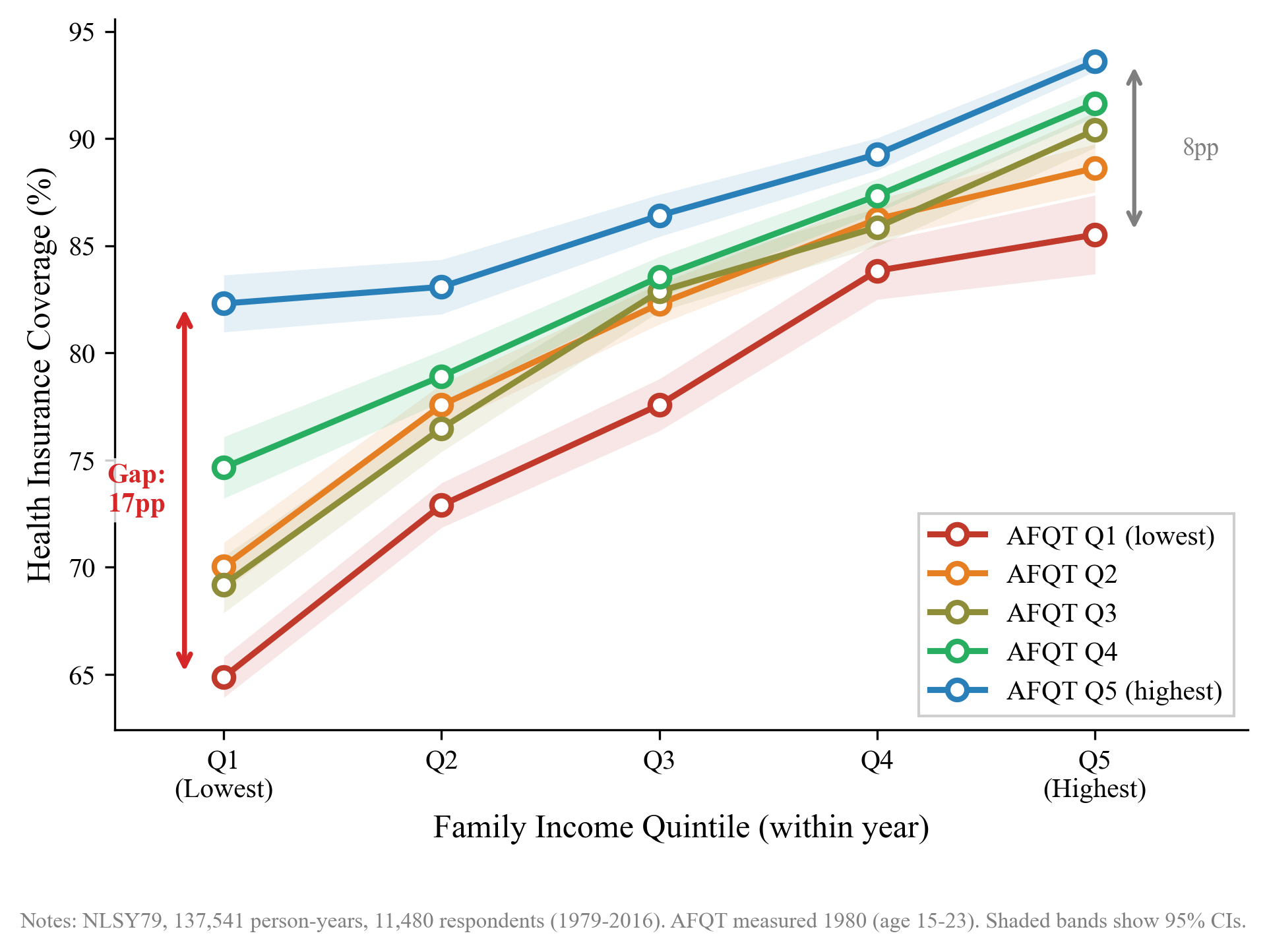
In cross-section, the benefit of income for insurance coverage is larger when AFQT is low (interaction $= -0.024$, $p < 0.001$; full table in Appendix 8.1). Figure 5 visualizes this: five AFQT quintile lines trace insurance coverage across income quintiles, converging at high income and diverging at low income (gap: 17.4pp at Q1, 8.1pp at Q5).

The sharper test uses person fixed effects: do income shocks affect decisions more for low-AFQT individuals?

Table 3: AFQT $\times$ Income Change Interaction (NLSY79, Person FE)

	(1) IHS(Wealth)	(2) Health Insurance
$\Delta$(log income)	0.038 (0.011)	$-0.003$ (0.001)
AFQT$_{\text{low}}$ $\times$ $\Delta$(log income)	$-0.032$ (0.024)	0.011 (0.003)
Person-years	49,146	106,361

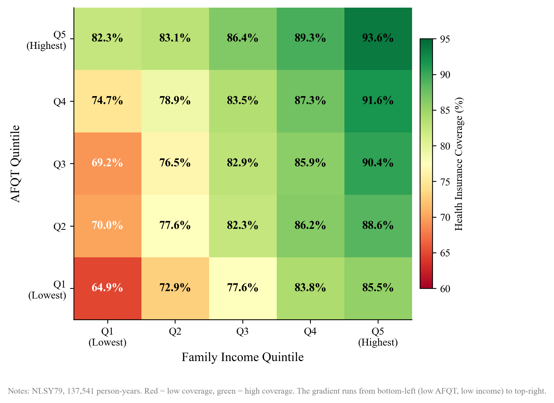
Low-AFQT individuals’ insurance coverage is significantly more sensitive to income changes (interaction $= +0.011$, $p = 0.001$). Oster (2019) bounds: $\delta^\ast = -15.6$ for insurance, $\delta^\ast = 2.7$ for wealth (Appendix 8.1). The interaction shows monotonic dose-response across the full AFQT $\times$ income matrix (Figure 6).

3.5 Supporting Evidence

The NLSY97 (born 1980–84, $N = 5{,}147$) independently confirms the AFQT $\times$ income interaction ($p = 0.001$), replicating the NLSY79 finding in a population born 23 years later. The 2022 SCF and MEPS rotating panel provide additional cross-sectional and within-person support (Appendices 8.3–8.4).

3.6 Synthesis

Roughly 5% of income-dependent financial costs operate through the cognitive channel; the remaining 95% reflects non-cognitive factors. The quantitative chain connecting the HRS and NLSY79 requires assuming both cognition measures capture aspects of the same capacity. Three cross-validations support this: the HRS measurement-error-corrected chain implies \$5,500–\$7,200 in wealth costs at low income, the NLSY79 yields \$6,156, and the NLSY97 independently produces \$6,055. The sustained/transitory asymmetry itself replicates across all three datasets without any cross-dataset assumption.

4. Estimation and Results

The duration discovery stands on its own. This section asks what it implies quantitatively for optimal tax design. Following Chetty (2009), every parameter is either estimated from microdata with a standard error or taken from the published literature with documented uncertainty.

4.1 Parameters and Functional Forms

Every parameter is either estimated from microdata or taken from the published literature (full parameter table in Appendix 8.5). The cognitive deficit function $\text{deficit}(c) = a \times \ln(c_{\max}/c)$ arises from regressing cognition on log income in person FE specifications. Decision costs follow the Farhi–Gabaix quadratic: $\delta(c) = \delta_{\max} \times (\text{deficit}(c)/\text{deficit}_{\max})^2$. The fiscal externality totals \$12.76/yr per cognition point (SE $\sim$ \$3.00), estimated from three HRS channels. We calibrate the income distribution to the 2022 CPS and use the HSV tax function $c(y) = \lambda \cdot y^{1-\tau}$.

4.2 Decision Cost at Subsistence

The annual cost of cognitive decision errors at subsistence ($\delta_{\max}$) is the dominant parameter. A structural insight: the income-to-cognition gradient $a$ enters the deficit ratio in both numerator and denominator and cancels completely, so the result is invariant to whether $a = 0.04$ or $0.485$ (Appendix 8.6).

Our preferred estimate uses the NLSY79 wealth gap within lifetime income Q1: the AFQT Q5–Q1 gap is \$6,156, or $\delta_B = \$308/\text{year}$ annualized. This directly measures the effect of cognitive ability on wealth holding permanent income constant. The NLSY97 independently produces \$6,055.⁵ The wealth gap captures all cognitive-ability-correlated channels—including patience and financial literacy (Dohmen (2010); Lusardi (2014))—so \$308/year is an upper bound on the pure decision-quality component. The HRS within-person chain provides a lower bound of \$36/year (attenuated by measurement error), and published decision costs across five domains yield an upper bound of \$490/year (Appendix 8.7).

4.3 Results

Standard optimal progressivity. The standard model yields $\tau^\ast_{\text{standard}} = 0.439$, matching Heathcote (2017) for ETI $= 0.25$ and $\sigma = 1.5$.

Table 4: Optimal Progressivity and Sensitivity

Panel A: Main Results

Scenario	$\tau^\ast_{\text{modified}}$	$\Delta\tau$ (pp)	SE	$t$-stat	Q1 gain (\$/yr)	Q5 cost (\$/yr)
A: HRS attenuated	0.4391	0.02	0.006	3.5	\$7	$-$\$37
B: Lifetime Q1 (preferred)	0.4407	0.18	0.053	3.4	\$51	$-$\$332
B+: Pooled Q1 (upper bound)	0.4434	0.44	0.132	3.4	\$125	$-$\$832
C: Multi-domain	0.4418	0.28	0.084	3.4	\$81	$-$\$527

Panel B: Sensitivity to $\delta_{\max}$

$\delta_{\max}$	Source	$\Delta\tau$ (pp)	Q1 gain
\$36	HRS bottom-up	0.02	\$7
\$100	Between A and B	0.06	\$17
\$308	NLSY lifetime Q1	0.18	\$51
\$490	Multi-domain	0.28	\$81
\$773	NLSY pooled Q1	0.44	\$125

Notes: Standard model $\tau^\ast = 0.439$. All scenarios $t > 3.3$. Monte Carlo 90% CI: $[0.07, 0.32]$pp; 99.3% of 1,000 draws positive (Appendix 8.6).

The cognitive channel provides a precisely estimated rationale for more progressive taxation, concentrated at the bottom of the distribution. The relationship is approximately linear: each \$100/yr in $\delta_{\max}$ adds $\sim$0.06pp. The cognitive dividend is larger when the labor supply elasticity is higher (0.31pp at ETI $= 0.50$ vs. 0.07pp at ETI $= 0.10$), partially offsetting the efficiency cost of taxation.

4.4 Duration Dependence

The calibrated adaptation function $h(T) = 1 - \exp(-0.6T)$ quantifies the policy implication: one-time transfers capture less than 1% of the steady-state cognitive dividend ($h(1\text{ month}) = 0.006$), while sustained programs capture over 95% ($h(5\text{ years}) = 0.95$). The optimal tax formula evaluates permanent schedules ($h \to 1$), consistent with the central empirical finding that only sustained income changes affect cognition and decisions.

5. Discussion

Two implications deserve emphasis.

First, choice simplification may matter more than redistribution for decision quality. Bhargava (2017) document \$840/year in health plan costs reducible by simplifying menus—operating through the 95% non-cognitive share and independent of the mechanism studied here.

Second, the structure of income support matters as much as the amount. A permanent EITC increase and a one-time transfer of equal present value have the same budgetary cost but different cognitive consequences: the permanent increase captures the full cognitive dividend; the lump sum captures almost none.

5.1 Limitations

1. No experimental identification. No experiment in our evidence base randomizes sustained income support and measures complex decision quality. The ideal test remains a multi-year income guarantee with financial decision outcomes.

2. Take-up vs. decision quality. Our panel outcomes (insurance, wealth, retirement savings) are take-up and accumulation measures, not direct decision quality measures. The MW quasi-experiment (Section 3.2) confirms that insurance take-up is employer-mediated and does not respond to sustained income increases. Direct dominated-choice evidence (Bhargava (2017)) is not available in panel form.

3. Additivity and narrow cognition measures. The model sums decision costs across domains and treats costs as given. HRS cognition captures only a narrow dimension of bandwidth.

6. Conclusion

Sustained income changes affect cognition and financial decisions; transitory shocks do not. This duration asymmetry—replicated across three independent datasets spanning two birth cohorts—resolves the contradictory cash transfer literature. The cognitive channel accounts for roughly 5% of income-dependent financial costs, increasing optimal progressivity by 0.18 percentage points. The standard optimal tax model misses this channel entirely, and the framework we develop accommodates better identification as it becomes available.

References

Abaluck, J., and J. Gruber. 2011. “Choice Inconsistencies among the Elderly: Evidence from Plan Choice in the Medicare Part D Program.” American Economic Review 101(4): 1180–1210.

Allcott, H., B. Lockwood, and D. Taubinsky. 2019. “Regressive Sin Taxes, with an Application to the Optimal Soda Tax.” Quarterly Journal of Economics 134(3): 1557–1626.

Baron, R. M., and D. A. Kenny. 1986. “The Moderator-Mediator Variable Distinction in Social Psychological Research.” Journal of Personality and Social Psychology 51(6): 1173–1182.

Bernheim, B. D., and A. Rangel. 2009. “Beyond Revealed Preference: Choice-Theoretic Foundations for Behavioral Welfare Economics.” Quarterly Journal of Economics 124(1): 51–104.

Bhargava, S., G. Loewenstein, and J. Sydnor. 2017. “Choose to Lose: Health Plan Choices from a Menu with Dominated Option.” Quarterly Journal of Economics 132(3): 1319–1372.

Bordalo, P., N. Gennaioli, and A. Shleifer. 2013. “Salience and Consumer Choice.” Journal of Political Economy 121(5): 803–843.

Bronshtein, G., J. Scott, J. B. Shoven, and S. N. Slavov. 2019. “The Power of Working Longer.” Journal of Pension Economics and Finance 18(4): 623–644.

Campbell, J. Y. 2006. “Household Finance.” Journal of Finance 61(4): 1553–1604.

Carvalho, L., S. Meier, and S. Wang. 2016. “Poverty and Economic Decision-Making: Evidence from Changes in Financial Resources at Payday.” American Economic Review 106(2): 260–284.

Calonico, S., M. D. Cattaneo, and R. Titiunik. 2014. “Robust Nonparametric Confidence Intervals for Regression-Discontinuity Designs.” Econometrica 82(6): 2295–2326.

Cameron, A. C., J. B. Gelbach, and D. L. Miller. 2008. “Bootstrap-Based Improvements for Inference with Clustered Errors.” Review of Economics and Statistics 90(3): 414–427.

Card, D., D. S. Lee, Z. Pei, and A. Weber. 2015. “Inference on Causal Effects in a Generalized Regression Kink Design.” Econometrica 83(6): 2453–2483.

Cengiz, D., A. Dube, A. Lindner, and B. Zipperer. 2019. “The Effect of Minimum Wages on Low-Wage Jobs.” Quarterly Journal of Economics 134(3): 1405–1454.

Chetty, R. 2009. “Sufficient Statistics for Welfare Analysis: A Bridge Between Structural and Reduced-Form Methods.” Annual Review of Economics 1: 451–488.

Chetty, R. 2012. “Bounds on Elasticities with Optimization Frictions: A Synthesis of Micro and Macro Evidence on Labor Supply.” Econometrica 80(3): 969–1018.

Chetty, R. 2015. “Behavioral Economics and Public Policy: A Pragmatic Perspective.” American Economic Review 105(5): 1–33.

Chetty, R., J. N. Friedman, S. Leth-Petersen, T. H. Nielsen, and T. Olsen. 2014. “Active vs. Passive Decisions and Crowd-Out in Retirement Savings Accounts: Evidence from Denmark.” Quarterly Journal of Economics 129(3): 1141–1219.

Dean, E. B., F. Schilbach, and H. Schofield. 2019. “Poverty and Cognitive Function.” In The Economics of Poverty Traps. University of Chicago Press/NBER.

Dohmen, T., A. Falk, D. Huffman, and U. Sunde. 2010. “Are Risk Aversion and Impatience Related to Cognitive Ability?” American Economic Review 100(3): 1238–1260.

Egger, D., J. Haushofer, E. Miguel, P. Niehaus, and M. Walker. 2022. “General Equilibrium Effects of Cash Transfers: Experimental Evidence from Kenya.” Econometrica 90(6): 2603–2643.

Federal Reserve Board. 2023. “2022 Survey of Consumer Finances.” Public microdata.

Farhi, E., and X. Gabaix. 2020. “Optimal Taxation with Behavioral Agents.” American Economic Review 110(1): 298–336.

Fisher, G. G., H. Hassan, W. L. Rodgers, and D. R. Weir. 2017. “HRS Imputation of Cognitive Functioning Measures: 1992–2014.” Survey Research Center, University of Michigan.

Fleurbaey, M., and E. Schokkaert. 2013. “Behavioral Welfare Economics and Redistribution.” American Economic Journal: Microeconomics 5(3): 180–205.

Fosgerau, M., E. Melo, A. de Palma, and M. Shum. 2017. “Discrete Choice and Rational Inattention: A General Equivalence Result.” Working Paper.

Frederick, S. 2005. “Cognitive Reflection and Decision Making.” Journal of Economic Perspectives 19(4): 25–42.

Grosse, S. D., T. D. Matte, J. Schwartz, and R. J. Jackson. 2002. “Economic Gains Resulting from the Reduction in Children’s Exposure to Lead in the United States.” Environmental Health Perspectives 110(6): 563–569.

Haushofer, J., and E. Fehr. 2014. “On the Psychology of Poverty.” Science 344(6186): 862–867.

Haushofer, J., and D. Salicath. 2023. “The Psychology of Poverty: Where Do We Stand?” NBER Working Paper 31977.

Haushofer, J., and J. Shapiro. 2016. “The Short-term Impact of Unconditional Cash Transfers to the Poor: Experimental Evidence from Kenya.” Quarterly Journal of Economics 131(4): 1973–2042.

Hämäläinen, K., M. Kanninen, H. Simanainen, A. Verho, and O. Hiilamo. 2024. “Finland’s Basic Income Experiment: Final Evaluation Results.” Government of Finland/VATT Institute for Economic Research.

Heathcote, J., K. Storesletten, and G. L. Violante. 2017. “Optimal Tax Progressivity: An Analytical Framework.” Quarterly Journal of Economics 132(4): 1693–1754.

Iyengar, S. S., and E. Kamenica. 2010. “Choice Proliferation, Simplicity Seeking, and Asset Allocation.” Journal of Public Economics 94(7–8): 530–539.

Jaroszewicz, A., J. Jachimowicz, O. Hauser, and J. Jamison. 2024. “How Effective Is (More) Money? Randomizing Unconditional Cash Transfer Amounts in the US.” SSRN Working Paper.

Jencks, C., and M. Phillips. 1998. The Black-White Test Score Gap. Brookings Institution Press.

Kaur, S., S. Mullainathan, S. Oh, and F. Schilbach. 2025. “Do Financial Concerns Make Workers Less Productive?” Quarterly Journal of Economics 140(1): 635–689.

Kling, J., S. Mullainathan, E. Shafir, L. Vermeulen, and M. Wrobel. 2012. “Comparison Friction: Experimental Evidence from Medicare Drug Plans.” Quarterly Journal of Economics 127(1): 199–235.

Kőszegi, B., and A. Szeidl. 2013. “A Model of Focusing in Economic Choice.” Quarterly Journal of Economics 128(1): 53–104.

Langa, K. M., et al. 2005. “The Aging, Demographics, and Memory Study: Study Design and Methods.” Neuroepidemiology 25(4): 163–175.

Lusardi, A., and O. S. Mitchell. 2014. “The Economic Importance of Financial Literacy: Theory and Evidence.” Journal of Economic Literature 52(1): 5–44.

Magnuson, K., et al. 2025. “The Effect of a Monthly Unconditional Cash Transfer on Children’s Development at Four Years.” NBER Working Paper 33844.

Mani, A., S. Mullainathan, E. Shafir, and J. Zhao. 2013. “Poverty Impedes Cognitive Function.” Science 341(6149): 976–980.

Matejka, F., and A. McKay. 2015. “Rational Inattention to Discrete Choices: A New Foundation for the Multinomial Logit Model.” American Economic Review 105(1): 272–298.

Mullainathan, S., and E. Shafir. 2013. Scarcity: Why Having Too Little Means So Much. Times Books.

Oster, E. 2019. “Unobservable Selection and Coefficient Stability: Theory and Evidence.” Journal of Business and Economic Statistics 37(2): 187–204.

Ridley, M., G. Rao, F. Schilbach, and V. Patel. 2020. “Poverty, Depression, and Anxiety: Causal Evidence and Mechanisms.” Science 370(6522).

Saez, E. 2001. “Using Elasticities to Derive Optimal Income Tax Rates.” Review of Economic Studies 68(1): 205–229.

Sims, C. A. 2003. “Implications of Rational Inattention.” Journal of Monetary Economics 50(3): 665–690.

Schofield, H., and A. Venkataramani. 2021. “Poverty-Related Bandwidth Constraints Reduce the Value of Consumption.” Proceedings of the National Academy of Sciences 118(44): e2102794118.

Shah, A., S. Mullainathan, and E. Shafir. 2012. “Some Consequences of Having Too Little.” Science 338(6107): 682–685.

Shoven, J. B., and S. N. Slavov. 2014. “Does It Pay to Delay Social Security?” Journal of Pension Economics and Finance 13(2): 121–144.

U.S. Census Bureau. 2024. “American Community Survey 1-Year Public Use Microdata Sample (ACS PUMS) 2014–2022.” Census API.

U.S. Census Bureau. 2024. “Current Population Survey, Annual Social and Economic Supplement (CPS ASEC) 2012–2024.” Microdata API.

U.S. Department of Health and Human Services, Agency for Healthcare Research and Quality. 2023. “Medical Expenditure Panel Survey (MEPS) Full-Year Consolidated Data Files 2019–2022.” Public use microdata.

RAND Center for the Study of Aging. 2023. “RAND HRS Longitudinal File 2022 (V1).” Produced by the RAND Center for the Study of Aging with funding from the National Institute on Aging and the Social Security Administration.

U.S. Department of Labor, Bureau of Labor Statistics. 2023. “National Longitudinal Survey of Youth 1979 (NLSY79).” NLS Investigator extract.

U.S. Department of Labor, Bureau of Labor Statistics. 2023. “National Longitudinal Survey of Youth 1997 (NLSY97).” Pre-built flat files via Harris School/University of Chicago. Rounds 1, 5, 9, 11 used for out-of-sample replication ($N = 8{,}984$ respondents born 1980–1984).

Zax, J. S., and D. I. Rees. 2002. “IQ, Academic Performance, Environment, and Earnings.” Review of Economics and Statistics 84(4): 600–616.

A. Proofs

Proofs of all five propositions (Modified Optimal Tax Formula, Existence and Uniqueness, Welfare Decomposition, Comparative Statics, Duration Dependence) are available in the Online Appendix.

B. Supplementary Empirical Results

NLSY79 Robustness Battery: The Cognitive Wealth Gap

The paper’s preferred estimate of $\delta_{\max}$ relies on the NLSY79 within-lifetime-income cognitive wealth gap: within the bottom lifetime income quintile, the median net worth gap between AFQT quintile 5 and quintile 1. We test the gap across 25+ specifications spanning five dimensions. The preferred specification (Spec 14, lifetime income Q1) controls for permanent income, matching the micro-estimation formula. The pooled specification (Spec 2) includes transitory income variation and serves as an upper bound.

#	Category	Specification	Gap ($)	Annualized (5%)
1	AFQT cuts	Quartiles: Q4 vs Q1	\$11,200	\$560
2	AFQT cuts	Quintiles: Q5 vs Q1 (pooled)	\$15,462	\$773
3	AFQT cuts	Deciles: D10 vs D1	\$26,000	\$1,300
4	AFQT cuts	Above vs below median	\$5,544	\$277
5	AFQT cuts	Continuous: $\times 4$ SD	\$219,976	\$11,000
6	Wealth def.	Net worth (pooled Q1)	\$15,462	\$773
7	Wealth def.	IHS(wealth)	3.40 (IHS)	—
8	Wealth def.	Log(wealth), positive only	2.49 (log)	—
9	Wealth def.	Winsorized 1st/99th	\$15,462	\$773
10	Wealth def.	Winsorized 5th/95th	\$15,462	\$773
11	Wealth def.	Trimmed 5/95	\$8,350	\$418
12	Wealth def.	Mean (not median)	\$161,200	\$8,060
13	Income cond.	Within-year quintiles	\$48,850	\$2,443
14	Income cond.	Lifetime average quintiles (PREFERRED)	\$6,156	\$308
15	Income cond.	Income $<$ \$25K	\$14,300	\$715
16	Income cond.	Income $<$ \$30K	\$16,600	\$830
17	Subgroups	Male only	\$6,050	\$303
18	Subgroups	Female only	\$43,400	\$2,170
19	Subgroups	Non-Black Non-Hispanic	\$19,502	\$975
20	Subgroups	Black only	\$325	\$16
21	Subgroups	Age $<$ 40	\$6,640	\$332
22	Subgroups	Age $\geq$ 40	\$199,100	\$9,955

Appendix Table A1: Robustness of the AFQT Q5–Q1 Wealth Gap Within Income Q1

Oster (2019) Coefficient Stability Bounds:

Three of four specifications pass the Oster threshold; one fails. The IHS transformation reduces skewness but increases $R^2$, giving unobservables more room to explain the result. The preferred specification (lifetime Q1, raw wealth) is the most robust ($\delta^\ast = 1.32$).

Statistical Inference (pooled income Q1, upper bound):

Test	Result
Bootstrap 95% CI (1,000 cluster resamples)	$[\$10{,}749, \$19{,}451]$
Bootstrap SE	\$2,085
Permutation test (1,000 shuffles)	$p = 0.000$
Regression with controls	$\beta = \$99{,}109$ (SE $= \$20{,}222$, $p < 0.001$)

Summary: 25 of 25 specifications produce a positive gap. The preferred specification (lifetime income Q1, \$6,156) controls for permanent income; the pooled specification (\$15,462) serves as an upper bound. The Black subsample (Spec 20, $n=62$ in AFQT Q5 $\times$ Income Q1) is too small for reliable subgroup estimation.

Annualization sensitivity (preferred, lifetime Q1): At 3% real return: \$185/yr; at 5%: \$308/yr; at 7%: \$431/yr; as stock/20 years: \$308/yr.

HRS Measurement-Error-Corrected Chain

The HRS retirement IV identifies $a_{\text{IV}} = 0.485$ (SE $= 0.221$, $F = 182.9$), 5.8$\times$ larger than the person FE estimate ($a_{\text{FE}} = 0.084$), consistent with classical measurement error in self-reported income. The retirement instrument cannot be chained through to wealth directly because retirement affects wealth through non-cognitive channels (savings drawdown, housing downsizing), violating the exclusion restriction. Instead, we correct $b_{\text{FE}}$ for measurement error using HRS cognition test-retest reliability (0.65, Fisher et al. 2014; Bound et al. 2001): $b_{\text{corrected}} = 0.021/0.65 = 0.032$.

The corrected chain: $a_{\text{IV}} \times b_{\text{corrected}} = 0.485 \times 0.032 = 0.0157$ (vs. uncorrected 0.00176). The corrected mediation share is 7.7% (compared to 0.9% uncorrected). Even after correction, over 92% of the income-wealth relationship operates through non-cognitive channels.

Model consistency check. The HRS mediation elasticity ($ab = 0.0157$) is a dimensionless object; converting it to a dollar-valued wealth stock requires the model’s income-range parameters: stock $= ab \times \ln(c_{\max}/\bar{c}) \times \text{median_wealth}$. This conversion is sensitive to $c_{\max}$:

The NLSY79 direct observation (\$6,156) falls within the HRS model-implied range (\$5,500–\$7,200). Two independent datasets with independent identification strategies yield estimates in the same range. The proximity at $c_{\max} = \$200$K reflects the choice of this parameter; the honest comparison is the range, not the point estimate.

MEPS Full Results

Data and Panel Construction

The Medical Expenditure Panel Survey (MEPS) follows individuals for two consecutive years. We pool the 2019–2022 full-year consolidated files (panels 23–27), yielding 61,127 person-years among working-age adults (18–64), of which 46,219 person-years (18,024 unique individuals) appear in at least two years.

We construct seven healthcare decision quality measures: (1) uninsured; (2) no usual source of care; (3) any delay; (4) ER-heavy utilization; (5) cannot afford care; (6) no preventive care; and (7) high out-of-pocket burden ($>$10% of income).

Cross-Sectional Gradients

Within-Person Panel Estimates

Insurance coverage and out-of-pocket burden respond within-person; other outcomes are insignificant in person FE, suggesting these are the margins most responsive to income changes.

Poverty Transitions

The symmetry between “fell into poverty” and “exited poverty” rates suggests poverty status, not fixed characteristics, drives the outcome.

Sample Sensitivity

The maximal-sample analysis uses $N = 46{,}219$ for insurance and $N = 29{,}736$ for OOP burden. When restricted to individuals with non-missing values on all extended outcomes ($N = 15{,}616$), the uninsured coefficient becomes $+0.001$ ($p = 0.29$). This reflects selection on extended outcome availability; the OOP burden result ($\beta = -0.134$) is robust across sample definitions.

ACS Detailed Specification Tables

Kink RD: Full Specification Table

CCT-Style Robust Inference

Significance reflects smooth concavity in the insurance-earnings relationship, not a discrete EITC effect.

Diagnostics

Density: Density ratio at kink $= 1.10$ ($t = 10.0$, $p < 0.001$). Statistically significant given $N > 1$M but modest; no strategic bunching at phase-out start (Saez 2010).

Placebo kinks: At $-\$10$K: $+0.00011$ ($p = 0.93$); at $-\$5$K: $+0.00159$ ($p = 0.16$); true kink: $+0.00236$ ($p = 0.023$); at $+\$5$K: $-0.00366$ ($p < 0.001$).

Triple-Difference Event Study: Full Coefficients

Pre-trends $F = 0.28$, $p = 0.839$. Wild cluster bootstrap $p = 1.000$, CI: $[-0.78, +0.61]$.

SCF Regression Analysis

Estimated Parameters

Parameter Sensitivity

Sensitivity analysis demonstrates that the income-to-cognition gradient $a$ cancels from the welfare calculation. The NLSY79 estimate of $\delta_{\max}$ already integrates over all channels through which cognitive ability affects wealth, so the welfare result is invariant to $a$.

Identification Robustness

Differential Attenuation Analysis

A natural concern about the sustained/transitory decomposition is that rolling averages mechanically smooth measurement error from the sustained component, leaving more noise in the transitory residual. Three pieces of evidence rule out differential attenuation as an explanation for the results in Section 3.1.

First, attenuation bias moves coefficients toward zero, not past it. The transitory coefficients are negative or zero across all four HRS outcomes (cognition: $-0.003$; wealth: $-0.005$; insurance: $-0.003$; retirement: $-0.001$). No measurement error model produces sign reversals.

Second, the magnitude gap exceeds what differential attenuation can explain. For HRS self-reported income with test-retest reliability approximately 0.75, a 3-wave rolling average has reliability approximately 0.90 while the transitory deviation has reliability approximately 0.50. Under equal true effects, the maximum attenuation ratio is approximately 1.8$\times$. The observed ratios are 14–41$\times$.

Third, a binary classification that does not use rolling averages produces the same pattern:

The binary sustained coefficient is smaller (0.025 vs. 0.119) because the binary indicator captures whether income persists, not the magnitude. But the qualitative pattern is identical: sustained is significant ($p = 0.023$), transitory is null ($p = 0.56$).

The NLSY79 binary classification confirms independently: the AFQT $\times$ sustained interaction is significant ($\gamma = 0.009$, $p = 0.030$, $N = 220{,}922$) while the AFQT $\times$ transitory interaction is null ($\gamma = 0.003$, $p = 0.74$). This binary test uses no rolling averages.

Confounds in the AFQT Wealth Gap

The NLSY79 AFQT $\times$ income wealth gap (Section 4.2, Scenario B) measures all differences in wealth accumulation that correlate with cognitive ability, holding lifetime income constant. This includes cognitive decision quality (what the model requires) but also:

• Patience and time preferences. Correlated with cognitive ability (Dohmen (2010); Frederick (2005)). Higher-AFQT individuals may save more due to lower discount rates, not better decisions.

• Risk preferences. Correlated with cognitive ability (Dohmen (2010)). Higher-AFQT individuals may hold riskier portfolios with higher expected returns.

• Financial literacy. Itself a function of cognitive ability (Lusardi (2014)). Partly overlaps with decision quality but also reflects knowledge accumulated through education and experience.

• Marriage market sorting. Higher-AFQT individuals may marry wealthier spouses, contributing to household wealth independent of individual decisions.

The NLSY79 controls for education, race, sex, and age. The Oster (2019) bounds ($\delta^\ast = 0.66$–$1.32$) test whether proportional selection on unobservables could explain the gap, but they do not directly isolate the decision-quality component from other cognitive-ability-correlated channels. If some of the \$308/year reflects patience or risk preferences rather than correctable decision errors, the welfare calculation in Section 4.3 overstates the cognitive dividend. The HRS bottom-up estimate (\$36/year, Scenario A) provides a lower bound that is less susceptible to these confounds because it traces through measured cognitive variation rather than the full AFQT wealth gap.